Vector Database Explained: Why Your AI App Needs One
You type “team meeting notes” into your company’s AI search tool. The document you’re looking for is titled “group standup summary.” You get zero results.
That failure is not a bug in your application logic. It’s a fundamental limitation of how traditional databases search. They match words. They don’t understand that “team meeting notes” and “group standup summary” mean the same thing.
Notion ran into this exact problem at scale. When they launched Notion AI Q&A in late 2023, they found that traditional keyword search missed semantically equivalent content constantly. Fixing it required a completely different kind of database — one that stores not the words themselves, but their meaning, encoded as numbers. That’s a vector database. And understanding how they work changes how you think about building AI features.
Table of Contents
What Are Vector Embeddings and Why Do They Matter?
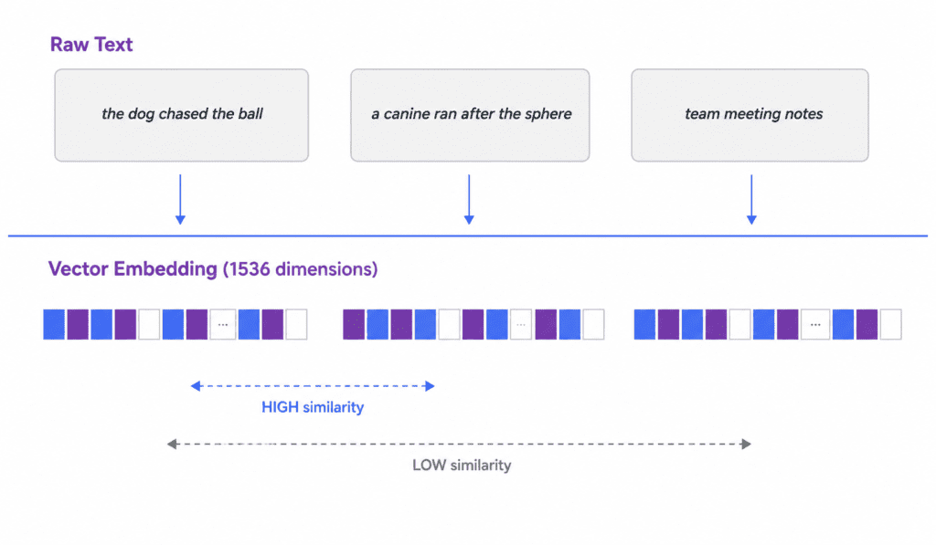
Before a vector database makes sense, embeddings need to make sense first. What are vector embeddings? They’re numerical representations of data like text, images, audio, anything where the numbers encode semantic meaning rather than literal content.
When a language model processes the sentence “the dog chased the ball,” it doesn’t store the letters. It produces a list of floating-point numbers — maybe 768 or 1536 of them — that collectively represent the meaning of that sentence in a high-dimensional space. These are the embeddings.
The geometric insight that makes vector databases useful: embeddings that mean similar things sit close together in that high-dimensional space. “Dog” and “canine” cluster near each other. “Dog” and “quantum physics” sit far apart. Similarity in meaning becomes measurable as distance between coordinates.
This is why vector databases can retrieve documents that mean the same thing as your query, even when they share zero words with it. They’re not searching text. They’re searching a geometric space where the distances between points reflect how related the underlying concepts are.
How closeness is measured depends on the application. Cosine similarity, which measures the angle between two vectors rather than the distance between their tips, is most common for text because it ignores the magnitude of the embedding and focuses purely on direction — useful when you care about semantic direction rather than how emphatically something was written. Euclidean distance and dot product are alternatives used for image and multimodal embeddings where magnitude carries information.
Semantic Search vs Keyword Search: What Actually Changes
Semantic search vs keyword search is the clearest way to understand why vector databases exist at all. Keyword search works on an inverted index: it maps words to the documents containing them, and query matching is exact. Ask for “heart attack” and you’ll only retrieve documents containing those exact words. “Myocardial infarction” — same medical condition — returns nothing.
Semantic search, powered by a vector database, asks a different question: not “which documents contain these words?” but “which documents are most similar in meaning to this query?” The query gets embedded just like the stored documents. Then the database finds the stored embeddings that are closest to the query embedding in geometric space.
A query for “heart attack” returns documents about myocardial infarction because their embeddings sit nearby. A query for “team meeting notes” returns documents about “group standup summaries” for the same reason.
The practical effect in production is significant. Notion’s engineering team reported that after deploying semantic search, they could retrieve content based on meaning rather than exact phrasing — which was the prerequisite for their AI Q&A feature to work at all. Keyword search simply could not surface relevant results when users phrased things differently from how the content was written, which is, of course, almost always.
How Approximate Nearest Neighbor Search Makes This Fast
Here’s the problem that took serious research to solve: if your vector database holds ten million 1536-dimensional embeddings, finding the closest one to a query by comparing all of them one by one would take seconds per query. That’s unusable.
Approximate nearest neighbor search (ANN) is the solution. Rather than guaranteeing the mathematically exact nearest neighbor, it finds something very close to the nearest neighbor, almost always within the top few results, in a fraction of the time. The “approximate” part sounds like a concession. In practice, for most applications, it isn’t — getting the 1st or 3rd closest result doesn’t meaningfully affect retrieval quality, but the speed difference between exact and approximate search is the difference between a 4-second query and a 4-millisecond one.
The dominant algorithm for ANN search today is called Hierarchical Navigable Small World graphs, or HNSW, published by Malkov and Yashunin and refined in a 2018 paper in IEEE Transactions on Pattern Analysis and Machine Intelligence (arXiv:1603.09320). Understanding the structure they designed explains why HNSW became the standard.
HNSW builds a multi-layer graph over the stored vectors. The bottom layer contains every vector in the database. Each vector’s presence in higher layers is determined randomly, with an exponentially decaying probability — so a small fraction of vectors appear in the second layer, an even smaller fraction in the third, and so on up to the top. The layers get progressively sparser as you go up.
Search works top-down. You enter at the top layer, which is sparse and coarse, and greedily navigate toward the region of the graph closest to the query vector. When you can’t get any closer in the current layer, you drop to the layer below, which is denser and more precise, and continue navigating. By the time you reach the bottom layer, you’ve already narrowed the search to a small local neighborhood, so only a handful of comparisons remain.
The consequence Malkov and Yashunin proved matters: this hierarchical design achieves logarithmic complexity scaling. In a flat brute-force search, doubling the dataset doubles the search time. With HNSW, doubling the dataset increases search time by roughly a single additional hop at the top layer. In production terms, this means a vector database serving ten million vectors isn’t dramatically slower than one serving one million. That scaling property is why HNSW has been adopted as the core indexing mechanism in Pinecone, Weaviate, Elasticsearch, and Qdrant.
When HNSW Isn’t the Right Index
One finding from a February 2026 benchmarking paper from UC Merced (Amanbayev et al., arXiv:2602.11443) complicates the “always use HNSW” advice that circulates in most tutorials. Their research evaluated how different indexing strategies perform when you combine vector search with metadata filters — for example, “find documents semantically similar to this query, but only from documents created after January 2025 by users in the engineering team.”
The results are counterintuitive for anyone who’s only read the HNSW marketing material. For highly selective filters — queries that constrain the search to a small fraction of the total index — partition-based indexes like IVFFlat outperform HNSW. The reason is structural: HNSW graphs are built assuming you’ll search the full dataset. When a filter eliminates 95% of the vectors before search, the graph structure that makes HNSW efficient breaks down. The greedy traversal is navigating a graph whose edges assume global connectivity, but you’re only allowed to land on a small island of valid vectors.
IVFFlat partitions vectors into clusters at index time. When filters are highly selective, you search only the relevant clusters — which turns out to be faster and more recall-stable than trying to adapt an HNSW graph to a heavily filtered subspace.
The practical guideline from that research: if your application does filtered search — and most real applications do, because users filter by date, category, user ID, document type, or metadata constantly — the choice between HNSW and IVFFlat isn’t obvious, and defaulting to HNSW because it’s the default in your chosen database isn’t always right. Match the index type to your query pattern, not to the algorithm’s benchmark headline.
The Index Is Just One Part of the Architecture
A vector database isn’t only an index. It’s a system that handles storage, updates, deletion, metadata filtering, access control, and query routing — all the things that make a search layer actually operable in production.
This is the distinction between a vector library like FAISS (Facebook AI Similarity Search) and a vector database like Pinecone, Chroma, or Weaviate. FAISS implements the ANN algorithms at high speed, but it doesn’t persist data to disk, doesn’t handle concurrent writes, and doesn’t manage metadata. You load vectors into memory, search them, and that’s it. It’s an excellent tool for research and prototyping, but it’s not a database.
Pinecone is a fully managed cloud service. You send it vectors and queries via API, and it handles the infrastructure completely. It’s the fastest path to production for teams that don’t want to run their own infrastructure. The trade-off is cost at scale and lack of self-hosting.
Chroma is open-source and designed for local development and smaller deployments. It’s the most common choice for developers building proof-of-concept RAG systems, because it runs in-process with zero infrastructure setup. The trade-off is that it doesn’t scale to billions of vectors.
Weaviate sits between the two. It’s open-source and self-hostable but also available as a managed cloud service, with more built-in features around data schema, multi-tenancy, and hybrid search (combining vector search with keyword-based BM25 search in a single query). For teams that need flexibility and plan to grow, Weaviate is often the longer-term choice.
The right pick depends on where you are. Chroma for local development. Pinecone if you want managed infrastructure immediately. Weaviate if you need schema control, hybrid search, or plan to self-host at scale.
Vector Databases for RAG: How the Pieces Connect
The most common reason teams add a vector database to their stack right now is to power retrieval-augmented generation. Vector databases for RAG applications work as the external memory that language models don’t have natively.
The setup: you take your documents — company knowledge base, product documentation, support tickets, whatever — chunk them into pieces, embed each chunk using an embedding model, and store those embeddings in a vector database. When a user asks a question, you embed the question the same way, retrieve the most similar document chunks from the database, and pass them as context to the language model alongside the question.
The model’s answer is now grounded in your actual documents, not just its training data. This is how you get a model to answer questions about your specific products, policies, or knowledge without fine-tuning it on your data. It also dramatically reduces hallucinations, because the model is working from retrieved facts rather than reconstructed memory.
The quality of the RAG system depends heavily on the vector database doing its job: returning the chunks that are genuinely most relevant to the question. If the retrieval is wrong, the model’s answer will be wrong regardless of how capable the model is. The RAG Explained post covers how the full pipeline fits together, including the chunking strategies and reranking steps that sit between the database and the model.
Understanding the role of the language model itself — what it can and can’t do without retrieval — is covered in the large language models explained post.
What This Doesn’t Cover
I left out quantization, specifically product quantization, which compresses embeddings to reduce memory cost at the expense of some recall accuracy. It becomes important at billion-vector scale but is irrelevant for most teams getting started. I also skipped hybrid search in detail — the combination of dense vector search and sparse keyword search (BM25) in a single query — which is worth a dedicated post once you’ve built a working vector search system.
FAQ
What is a vector database in simple terms?
A vector database stores data as numerical coordinates — called embeddings — in a high-dimensional space, where similar items sit close together geometrically. Instead of matching keywords, it finds items closest in meaning to your query. This lets you search by concept, not just by exact word, which is why it’s the foundation of semantic search and AI memory systems.
Do I need a vector database to build a RAG system?
For prototyping: not strictly. You can run FAISS in memory for small document collections. For anything production-scale — more than a few tens of thousands of documents, multiple users, or documents that update frequently — you need a proper vector database that handles persistence, concurrent writes, and filtered retrieval. Chroma is the standard starting point; Pinecone or Weaviate when you need scale or managed infrastructure.
What’s the difference between Pinecone, Chroma, and Weaviate?
Pinecone is a fully managed cloud service — zero infrastructure work, fastest time to production, higher cost at scale. Chroma is open-source and runs locally, ideal for development and small deployments. Weaviate is open-source and self-hostable with a managed cloud option, offering more schema control, hybrid search, and multi-tenancy for teams building larger systems. Start with Chroma, move to the other two when you have a reason to.
The reason vector databases matter right now is that most of the interesting AI applications- search that understands questions, assistants that know your documents, recommendation systems that match intent- depend on moving from exact-match retrieval to meaning-based retrieval. The database is what makes that shift possible in production, not just in demos.
The piece most tutorials miss is that the indexing algorithm you choose has real consequences at scale, and those consequences aren’t always what the benchmarks suggest. Know what HNSW is optimizing for — and when to reach for something else.