Convolutional Neural Networks: How Machines Learn to See

You pull your phone out of your pocket. Before you’ve pressed a single button, it recognises your face and unlocks. The whole thing takes about 300 milliseconds.

Somewhere inside that 300 milliseconds, a convolutional neural network is scanning your face pixel by pixel, detecting the curve of your jaw, the distance between your eyes, the slope of your nose, and matching that spatial pattern against a stored representation of you — all without a single human-written rule about what a face is.

That’s the part worth understanding. The network was never told what a face looks like. No engineer encoded “eyes are round” or “faces are symmetric.” The network looked at millions of images, and through the mathematics of convolution and backpropagation, it figured all of that out on its own.

Here’s exactly how.

Why Regular Neural Networks Fail on Images

Before getting into convolutions, it’s worth understanding why a standard neural network can’t solve image classification efficiently.

A typical neural network works by connecting every input to every neuron in the first layer. For a small 224×224 colour image, that’s 224 × 224 × 3 = 150,528 input values. Connect each one to even a modest first layer of 1,000 neurons and you immediately have 150 million parameters — just in the first layer. Train on slightly larger images and you’re in the billions. The network becomes computationally unworkable and is almost guaranteed to overfit, because it has far more parameters than meaningful patterns to learn.

The deeper problem isn’t just scale. A fully connected network treats every pixel as independent of every other pixel. It has no concept of spatial structure. Shifting a cat three pixels to the right produces a completely different input vector, even though it’s obviously still the same cat. A standard network would have to re-learn “cat” from scratch for every possible position, rotation, and scale.

Convolutional neural networks solve both problems at once. The architecture was designed specifically around the structure of visual data.

The Core Insight: Local Connectivity and Weight Sharing

The foundational CNN architecture, LeNet-5, was introduced by Yann LeCun, Léon Bottou, Yoshua Bengio, and Patrick Haffner in their 1998 paper “Gradient-Based Learning Applied to Document Recognition” (Proceedings of the IEEE). The insight that paper formalised had been percolating in LeCun’s work since 1989, but the 1998 paper demonstrated it at scale on the handwritten digit recognition problem.

The core idea is this: instead of connecting every input pixel to every neuron, connect each neuron only to a small local region of the image. A neuron in layer 1 looks at a 5×5 patch of pixels. Another neuron looks at the adjacent 5×5 patch. Each one is only responsible for detecting patterns in its local neighbourhood.

This is called local connectivity, and it directly mirrors how the visual cortex works. Individual neurons in the visual cortex respond to stimuli only in a restricted region of the visual field, called the receptive field. LeCun’s architecture made the same choice for computational reasons, but it turns out to be biologically motivated as well.

The second principle is weight sharing. Rather than each neuron in a layer learning its own independent set of weights, all neurons in the same layer share the same weights. This shared set of weights is called a filter (or kernel). One filter slides across the entire image, applying the same transformation at every location.

Why does this work? Because useful visual features like edges, corners, and colour gradients appear throughout images, not just in one fixed location. A vertical edge detector is useful whether the edge appears on the left side or the right side of the image. Weight sharing lets the network learn one edge detector and apply it everywhere, rather than learning a separate edge detector for every possible position.

The result: dramatically fewer parameters, and a network that gains something called translational invariance — the same filter fires whether the feature appears top-left or bottom-right.

What Filters Actually Learn (The Research Answer, Not the Textbook Answer)

Most explanations say filters detect edges, then textures, then shapes — and leave it there. That’s true, but it’s incomplete. The more interesting question is: how do we know that’s what they learn?

The answer came from Matthew Zeiler and Rob Fergus in their 2013 paper “Visualizing and Understanding Convolutional Networks” (arXiv:1311.2901, presented at ECCV 2014). The paper introduced a deconvolutional network technique: a way to project activations from any layer back down to pixel space, revealing what input pattern caused a particular filter to fire maximally.

What they found was striking. The hierarchy wasn’t just intuitive — it was measurable and consistent across different networks:

Layer 1 filters respond to oriented edges and colour blobs. These are the most primitive visual features — a diagonal line here, a blue-to-green gradient there.

Layer 2 filters respond to textures and corners: grid patterns, repeating structures, L-shaped junctions. These are combinations of the edges from layer 1.

Layer 3 filters respond to more complex patterns: mesh-like textures, repeating motifs, the beginning of recognisable objects like wheels or faces in abstract form.

Layers 4 and 5 respond to class-specific features. Zeiler and Fergus showed that by layer 4, filters are firing on dog faces, keyboard textures, and text characters. The network has, entirely from data, learned to assemble primitive edges into meaningful object parts.

This wasn’t designed in. It emerged from training on images. That’s the part that still feels remarkable if you sit with it.

The Zeiler/Fergus paper also showed something practically important: you could take a network trained on ImageNet, remove its final classification layer, retrain just that layer on a completely different dataset (Caltech-101, Caltech-256), and get state-of-the-art performance with very few training images. The learned features generalised. This was early evidence for what would become the transfer learning paradigm, which I cover in detail in the transfer learning post.

The Mechanics: Filters, Feature Maps, Pooling, Stride, Padding

With the “why” covered, here’s how each component works in practice.

Filters are small matrices — typically 3×3 or 5×5 — filled with learnable weights. During training, these weights are updated via backpropagation to detect increasingly useful patterns. At the start of training, filters are initialised randomly. By the end, they’ve converged to the edge and texture detectors described above.

Feature maps are the outputs of applying a filter to the input. If you apply a 3×3 filter to a 32×32 image by sliding it across every position, you get a 30×30 output map (assuming no padding) showing where and how strongly that filter activated. A convolutional layer typically applies dozens or hundreds of different filters in parallel, producing dozens or hundreds of feature maps — each representing a different detected pattern.

import torch
import torch.nn as nn

# A single convolutional layer: 32 filters, each 3x3, applied to a 3-channel image
conv_layer = nn.Conv2d(in_channels=3, out_channels=32, kernel_size=3, stride=1, padding=1)

# Input: batch of 8 images, 3 channels, 224x224
x = torch.randn(8, 3, 224, 224)
output = conv_layer(x)

print(output.shape)  # torch.Size([8, 32, 224, 224])
# 32 feature maps, same spatial size due to padding=1

Stride controls how far the filter moves at each step. Stride 1 means the filter moves one pixel at a time, creating a dense output. Stride 2 means it jumps two pixels, halving the spatial dimensions. Higher strides reduce output size and computation, at the cost of finer spatial detail. Stride is often used instead of pooling in modern architectures to control downsampling.

Padding adds zeros around the border of the input before applying the filter. Without padding, each convolution operation shrinks the spatial dimensions slightly. In a deep network with many layers, this shrinkage compounds until you’ve lost most of your spatial resolution. “Same” padding adds just enough zeros to keep output dimensions equal to input dimensions. This is especially important in deep networks where spatial resolution matters.

Pooling reduces spatial dimensions by summarising regions of a feature map. Max pooling takes the maximum value from each region, keeping the strongest activation. Average pooling takes the mean. A 2×2 max pooling operation with stride 2 halves the spatial dimensions, reducing computation and memory. Importantly, pooling provides a form of local translational invariance: if a detected feature shifts by one pixel, the max pooling output doesn’t change.

AlexNet (2012) used max pooling with overlapping regions — a deliberate design choice the authors noted helped with regularisation. LeNet-5 (1998) used average pooling. Modern architectures often replace pooling with strided convolutions entirely.

The 2012 Moment: When CNNs Proved It at Scale

Understanding why CNNs matter requires knowing what happened in 2012. The ImageNet Large Scale Visual Recognition Challenge (ILSVRC) was an annual benchmark competition for image classification on a dataset of over a million images across 1,000 categories. The best methods in 2010 and 2011 were hand-crafted feature engineering pipelines, achieving top-5 error rates around 26%.

In 2012, Alex Krizhevsky, Ilya Sutskever, and Geoffrey Hinton entered a convolutional neural network they called AlexNet. It achieved a top-5 error rate of 15.3% — an improvement of nearly 11 percentage points over the previous best, a margin so large it was initially suspected to be a mistake in the results.

The AlexNet architecture (Krizhevsky et al., NIPS 2012) had five convolutional layers followed by three fully connected layers. But the architectural choices mattered as much as the depth:

ReLU activations replaced sigmoid and tanh nonlinearities. ReLU trains several times faster than tanh because it doesn’t saturate for large positive values, which keeps gradients healthy during backpropagation. This was borrowed from earlier work but applied at scale for the first time.

Dropout was applied in the fully connected layers. By randomly deactivating half the neurons during each training step, the network couldn’t rely on any single pathway and was forced to learn redundant, robust representations.

GPU training reduced training time from weeks to days, making the scale of the experiment feasible.

The lower convolutional layers of AlexNet learned oriented edges and colour blobs — essentially the same primitive features LeNet-5 had learned on handwritten digits 14 years earlier. The higher layers learned dog faces, keyboards, and object-specific textures. The hierarchy LeCun described in 1998 held up at ImageNet scale.

The Degradation Problem and Why Deeper Isn’t Always Better

The natural response to AlexNet’s success was: add more layers. If eight layers gets 15% error, surely 30 layers gets lower? Researchers tried. The results were paradoxical.

Adding more layers to a plain convolutional network made it worse, not better. This is now called the degradation problem: as depth increases beyond a certain point, training accuracy itself degrades, even with batch normalisation. The network becomes harder to optimise.

He, Zhang, Ren, and Sun at Microsoft Research identified the cause and published the solution in “Deep Residual Learning for Image Recognition” (arXiv:1512.03385, CVPR 2016). Their insight: rather than asking each layer to learn a full transformation from input to output, make each layer learn only the residual — the difference between the input and the desired output.

Concretely, this means adding a shortcut connection that skips one or more layers and adds the input directly to the output:

class ResidualBlock(nn.Module):
    def __init__(self, channels):
        super().__init__()
        self.conv1 = nn.Conv2d(channels, channels, 3, padding=1)
        self.bn1   = nn.BatchNorm2d(channels)
        self.relu  = nn.ReLU()
        self.conv2 = nn.Conv2d(channels, channels, 3, padding=1)
        self.bn2   = nn.BatchNorm2d(channels)

    def forward(self, x):
        residual = x                          # save input
        out = self.relu(self.bn1(self.conv1(x)))
        out = self.bn2(self.conv2(out))
        out += residual                       # add input back
        return self.relu(out)

If the optimal transformation for a block is close to the identity function (do nothing), a residual connection makes this trivially easy to learn: just push the weights toward zero. Without skip connections, learning the identity function through stacked nonlinear layers is surprisingly hard.

ResNet-152 — 152 layers deep, eight times deeper than AlexNet — achieved 3.57% top-5 error on ImageNet, winning ILSVRC 2015 across classification, detection, and localisation categories simultaneously. ResNet’s residual connections have since become a standard component in virtually every modern deep learning architecture, including transformers.

Object Detection and Beyond Image Classification

Image classification asks “what is in this image?” and returns a single label. Object detection asks “what is in this image, and where?” and returns both labels and bounding boxes.

CNN-based object detection architectures like R-CNN, Fast R-CNN, and YOLO use the same convolutional feature extraction principles but add spatial prediction heads. Rather than pooling all feature maps into a single class label, they preserve spatial information and predict object locations from different regions of the feature map.

The intuition is the same: early layers detect edges and textures, middle layers detect object parts, final layers have enough context to say “there’s a person at this position in the image.” The convolutional feature hierarchy is doing the same work in both tasks.

What CNNs Can’t Do (The Honest Part)

CNNs have a real weakness that’s worth understanding: they’re brittle to distribution shift, and they can be fooled by adversarial examples in ways that reveal something fundamental about what they’ve learned.

A small, carefully constructed perturbation to an image — one invisible to the human eye — can cause a CNN to confidently misclassify a cat as a guacamole bowl. The network hasn’t learned “what a cat is” in any deep sense. It’s learned a set of statistical correlations between pixel patterns and labels. When those correlations are exploited, the model fails.

This matters for deployment. A CNN trained on photographs may perform poorly on images taken with a different camera. A CNN trained on one hospital’s CT scans may degrade when applied to scans from a different scanner model. The spatial hierarchy the network learns is real and powerful, but it’s not the same as understanding.

For most practical applications, transfer learning sidesteps the worst of this problem: pretrained models have seen enough diversity to generalise reasonably. If you want to understand how to use that effectively, the transfer learning post covers feature extraction vs. fine-tuning in detail.

For the mathematical relationship between depth, representation power, and generalisation — the principles that explain why CNNs work at all — Stanford’s CS231n lecture notes on Convolutional Networks remain the most rigorous publicly available treatment.

FAQ

The thing that’s stayed with me from reading through the original papers: LeCun’s 1998 architecture, trained on handwritten zip codes at AT&T, and the ResNet winning ILSVRC 2015 by detecting objects in millions of real-world photographs — they’re running the same idea. Local connectivity, weight sharing, learned hierarchical features. Twenty years and several orders of magnitude of scale separate them, but the conceptual core is the same.

Which either means the idea was right the first time, or it means we’ve been building on a very narrow set of assumptions for a long time. Probably both.

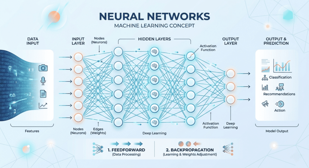
If you want to understand how CNNs fit into the broader picture of how neural networks learn, the neural networks explained post is the right starting point before going deeper into architecture specifics.