Naive Bayes Classifier Explained: Why the Naive Assumption Keeps Working

The standard explanation for why Naive Bayes works is unsatisfying. It usually goes: “Yes, the independence assumption is violated, but somehow it still works in practice. Isn’t that interesting?” And then the post moves on to the math.

That’s not an explanation. It’s a shrug with a LaTeX equation underneath it.

The real answer is more precise and, honestly, more interesting. Whether feature dependencies hurt Naive Bayes performance has less to do with how correlated your features are and more to do with a different property entirely — one that an IBM Research study spent considerable effort establishing through Monte Carlo simulation. Getting that distinction right changes how you think about when to use this algorithm and when to abandon it.

What Naive Bayes Actually Does

Before getting into why it works, the mechanics need to be clear.

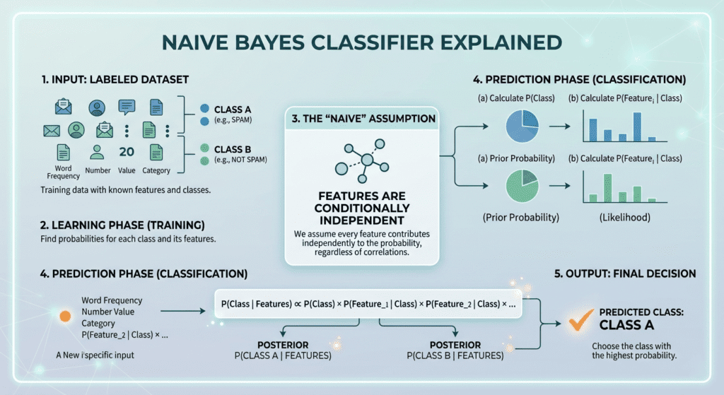
Naive Bayes is a probabilistic classifier built on Bayes’ theorem. Given a new observation with features, you want to know the most probable class. Bayes’ theorem gives you the framework:

P(class | features) ∝ P(features | class) × P(class)

In plain terms: the probability of a class given your data is proportional to how likely that data is if the class were true (the likelihood), multiplied by how common that class is in the training data (the prior probability).

To classify a new example, you compute this quantity for every class and pick the highest one. The class with the most probability wins.

The problem is computing P(features | class) for a real dataset. If you have 20,000 vocabulary terms in a text classifier, computing the joint probability of every possible combination of words appearing is computationally infeasible. Manning, Raghavan, and Schütze worked through this in their foundational text on information retrieval: for a binary Bernoulli model with M vocabulary terms, you’d need to estimate 2^M parameters per class — one for every possible combination of term presence and absence. With even a modest vocabulary, that number exceeds the number of atoms in the observable universe.

This is the actual origin of the independence assumption, and it’s worth understanding it this way: the assumption doesn’t exist because anyone thought it was true. It exists because it makes the computation tractable. By assuming conditional probability independence among features given class, the joint probability collapses into a simple product of individual term probabilities. The number of parameters drops from exponential to linear in the vocabulary size.

Definition: The Naive Bayes classifier assigns a class to an observation by computing the posterior probability of each class given the observed features, using Bayes’ theorem combined with the conditional independence assumption. Each feature’s likelihood contribution is estimated separately and multiplied together, which makes the computation linear in the number of features rather than exponential.

So the naive assumption was never a claim about reality. It was a computational bargain. The interesting question is why that bargain turns out to work as well as it does.

The Probability Paradox at the Heart of Naive Bayes

Stanford’s IR textbook makes a distinction that most treatments skip entirely: there’s a difference between estimating probabilities correctly and making correct classification decisions. Naive Bayes does one of these things badly and the other surprisingly well.

The probability estimates Naive Bayes produces are typically wrong. Not slightly wrong — badly wrong. When a document clearly belongs to a class, Naive Bayes often assigns it a probability of 0.99 when the true posterior might be 0.60. The model is overconfident, because it multiplies likelihoods across features that aren’t actually independent, double-counting evidence. A document about Beijing that mentions “China” three times has that evidence counted three times as if each mention were independent information about a different aspect of the document.

But here’s the thing: classification doesn’t need accurate probabilities. It needs the right class to come out on top. And as long as the right class produces a larger (even if badly calibrated) score than all the other classes, the decision is correct. Manning and colleagues illustrate this with a concrete example: a document with true posteriors of 0.6 for class 1 and 0.4 for class 2 might produce Naive Bayes estimates of 0.99 and 0.01 respectively. The estimates are wildly off. The decision — class 1 — is exactly right.

Correct estimation implies accurate prediction, but accurate prediction does not require correct estimation. Naive Bayes exploits this gap. It’s a bad probability estimator that happens to be a good classifier.

This distinction has a practical consequence: if you need calibrated probability outputs (for risk scoring, medical diagnosis confidence, anything where the magnitude of the probability matters), Naive Bayes probabilities need calibration post-hoc. Raw Naive Bayes probabilities should not be trusted as literal probabilities. If you only need the classification decision, they work fine as-is.

The Real Question: When Does Naive Bayes Break?

Most explanations of Naive Bayes failures say: “it breaks when features are correlated.” That’s too coarse to be useful. Irina Rish’s empirical study at IBM T.J. Watson Research Center ran Monte Carlo simulations across thousands of randomly generated classification problems and found something that contradicts the standard narrative.

The degree of feature dependency — measured as class-conditional mutual information between features — is not a reliable predictor of Naive Bayes error. You cannot look at a correlation matrix and infer whether Naive Bayes will struggle.

What is a better predictor is information loss: how much of the class-relevant information contained in the features is lost when you apply the independence assumption. Two highly correlated features might both be carrying the same information about the class, in which case Naive Bayes double-counts that information but still arrives at the right decision. Two features with moderate correlation might carry different class-relevant information that the independence assumption conflates in a damaging way.

The practical implication: Naive Bayes performance follows a U-shaped curve with respect to feature dependency. It performs well when features are genuinely independent, as you’d expect. But it also performs well when features are fully functionally dependent — when one feature is a deterministic function of another. In that case, the model double-counts evidence, but does so symmetrically across classes, so the rank ordering is preserved and classification remains correct.

The worst performance occurs in between: moderate, non-functional dependencies where features share partial class-relevant information in an asymmetric way that distorts the ranking. This is more common in tabular data with engineered features than in raw text, which is part of why Naive Bayes has an unusually strong track record on text classification and a spottier one on general tabular data.

How the Algorithm Actually Learns

Training a Naive Bayes classifier is embarrassingly simple. You go through your training data, count how often each feature value appears per class, compute the relative frequencies, and store those as your likelihood estimates. The prior probability for each class is just its fraction of the training set. That’s the entire training process — one pass through the data.

from sklearn.naive_bayes import MultinomialNB, GaussianNB
from sklearn.feature_extraction.text import CountVectorizer
from sklearn.pipeline import Pipeline

# Text classification (spam filter example)
pipeline = Pipeline([
    ('vectorizer', CountVectorizer()),
    ('classifier', MultinomialNB(alpha=1.0))  # alpha is Laplace smoothing
])

pipeline.fit(X_train_text, y_train)
predictions = pipeline.predict(X_test_text)
predicted_probs = pipeline.predict_proba(X_test_text)
# Remember: these probabilities are poorly calibrated — use for ranking, not literal probabilities

One detail worth understanding: alpha=1.0 applies Laplace smoothing. Without it, any word that appears in test data but not in training data for a given class produces a zero likelihood, which zeros out the entire product for that class regardless of all other evidence. Laplace smoothing adds a small count to every word-class combination to prevent this, which is why real spam filter implementations always include it.

Gaussian Naive Bayes: When Features Are Continuous

The multinomial version works for count data. For continuous features — sensor readings, measurements, anything that isn’t a word count — Gaussian Naive Bayes applies a different likelihood model.

Instead of counting occurrences, Gaussian NB assumes the values of each feature within each class follow a normal (Gaussian) distribution. It estimates the mean and variance of each feature per class from training data, then uses the Gaussian probability density function as the likelihood term.

from sklearn.naive_bayes import GaussianNB

gnb = GaussianNB()
gnb.fit(X_train, y_train)

# Inspect what the model learned
print(gnb.theta_)    # class-conditional means for each feature
print(gnb.var_)      # class-conditional variances for each feature

The Gaussian assumption creates its own constraint: it works well when features within each class really are roughly bell-shaped. Log-transform heavily skewed features before using Gaussian NB. For count data, stick with Multinomial NB. For binary presence/absence features, Bernoulli NB (which estimates term occurrence probabilities per class rather than term frequencies) is the correct choice. Mixing these up is a common implementation error that produces quietly bad results.

Where Naive Bayes Still Earns Its Place

The text classification and spam filter use cases are well-established. For a spam classifier, the relevant question is whether certain word combinations appear more in spam than in ham. The independence assumption says “free” and “money” each carry independent information, which they don’t — but both are spam indicators, their double-counting pushes spam probability higher than ham, and the classifier gets it right anyway. This is the U-shaped curve in practice: the functional dependence between spam-correlated words doesn’t hurt because it’s symmetric.

Naive Bayes also handles high-dimensional feature spaces efficiently in ways that matter at scale. Training on a million documents with a 50,000-word vocabulary is a pass through the data. Inference is a multiplication chain. No gradient descent, no iterative optimization, no convergence monitoring. The speed advantage over more sophisticated classifiers can be meaningful when classification latency matters or when retraining frequency is high.

The feature engineering connection is worth noting here. The quality of features fed to Naive Bayes directly determines the quality of its likelihood estimates. Because the classifier relies purely on frequency statistics, irrelevant features dilute the signal rather than being ignored the way tree-based models can ignore them. Proper feature selection before applying Naive Bayes — removing features with no class-predictive power — often matters more than it does for other algorithms. The feature engineering post covers the relevant selection techniques in detail.

Where Naive Bayes doesn’t hold up: when you need well-calibrated probabilities, when features have complex non-functional interactions that carry different information per class, or when the decision boundary in feature space is genuinely nonlinear in a way the independence assumption can’t approximate.

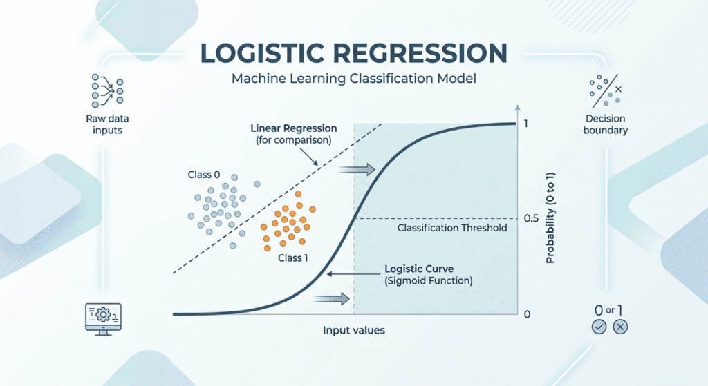
Logistic regression solves many of the same text classification problems with better-calibrated outputs and the ability to learn feature weights that account for correlations — at the cost of more data and slower training. For a direct comparison of when to choose one over the other, the logistic regression post covers the decision boundary and calibration differences in depth.

Practical Decision Guide

Use Naive Bayes when:

• Your features are word counts, term frequencies, or binary presence/absence indicators
• Training data is limited and you need a stable model
• Training or inference speed is a hard constraint
• You want a fast, interpretable baseline before trying heavier algorithms

Switch to something else when:

• You need calibrated probability outputs and can’t add a calibration layer
• Features are continuous with non-Gaussian distributions within classes
• Feature interactions are complex and asymmetric (tabular data with many engineered features)
• You have enough data that a more flexible model like logistic regression or gradient boosting would meaningfully outperform

The scikit-learn Naive Bayes documentation covers all three variants (Multinomial, Bernoulli, Gaussian) with their appropriate use cases and implementation details.

FAQ