Logistic Regression: Not a Regression at All – Here’s What It Actually Does

The name is wrong. That’s not a hot take. That’s the actual history.

When David Cox published “The Regression Analysis of Binary Sequences” in 1958, he was solving a specific problem: how do you model the probability that a binary outcome depends on one or more independent variables? His answer was to take a linear combination of features and pass it through a function that squashes the output into the range [0, 1]. The word “regression” stuck because the linear part of the model looks like regression. But what the algorithm actually does is classification. It estimates the probability that a given input belongs to one class or another, and then you draw a line somewhere in that probability space and say everything above it is a “yes.”

Sixty-seven years later, logistic regression still powers a significant slice of real production classification systems. Spam filters. Credit scoring. Medical diagnosis screening. Not because teams don’t know about gradient boosting or neural networks. Because when your features are reasonable, your classes aren’t wildly imbalanced, and you need to explain the model’s decisions to a human being, logistic regression is genuinely hard to beat.

But here’s the thing nobody tells you: most people who use it are misreading its output. The coefficients don’t mean what you think they mean. The 0.5 decision threshold is almost always wrong. And the model isn’t fitting a curve at all. Understanding those three things is the difference between using logistic regression correctly and getting confidently wrong answers.

What the Algorithm Is Actually Doing

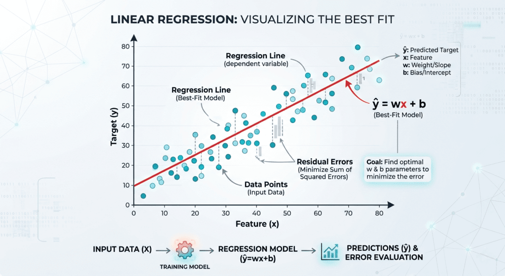
Start with linear regression. You’ve got a set of features, you multiply each by a learned weight, add them up, and get a prediction. That prediction can be any real number, from negative infinity to positive infinity, which is fine when you’re predicting house prices but catastrophic when you’re predicting probability. Probability has to live between 0 and 1. You can’t have a 140% chance of a loan defaulting.

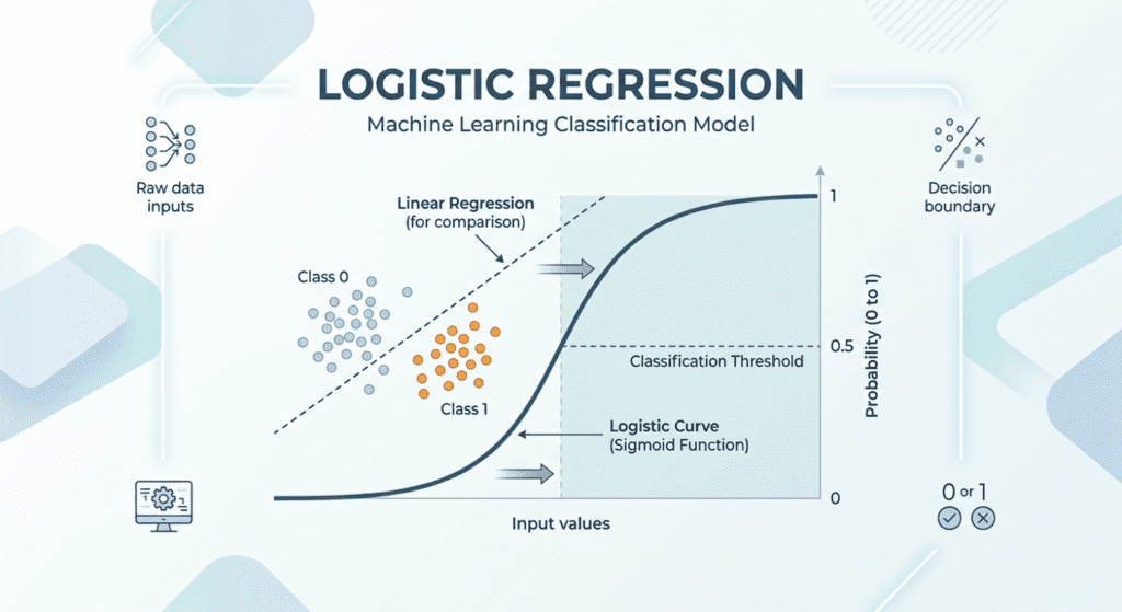
The sigmoid function solves this. It takes any real number as input and outputs a value between 0 and 1. The formula is σ(z) = 1 / (1 + e^(-z)). At z = 0, it outputs 0.5. Push z toward positive infinity and it approaches 1. Push it toward negative infinity and it approaches 0. The S-shaped curve it traces is where the “logistic” in logistic regression comes from.

So logistic regression does exactly what linear regression does with the weighted sum, but then passes that sum through the sigmoid to produce a probability. The model outputs: “given these features, there’s a 73% chance this email is spam.” You then decide what to do with that probability.

Definition: Logistic regression is a supervised classification algorithm that models the probability of a binary outcome by passing a linear combination of input features through a sigmoid function. Despite the name, it’s a classification algorithm. It was developed by statistician D.R. Cox in 1958 to model binary dependent variables.

The math underneath is using log-odds (also called logits) as the linking mechanism. The model is actually fitting a linear relationship between your features and the logarithm of the odds ratio: log(p / (1-p)). This is why the raw coefficients the model learns are in log-odds units, not probability units. That distinction matters more than most tutorials acknowledge.

The Coefficient Interpretation Problem

Here’s where most logistic regression explanations quietly go wrong.

In linear regression, a coefficient of 0.3 on a feature means: every one-unit increase in that feature increases the predicted output by exactly 0.3, regardless of what the other features are doing. The relationship is direct and constant.

In logistic regression, a coefficient of 0.3 on a feature does not mean “a one-unit increase raises the predicted probability by 0.3.” It means a one-unit increase raises the log-odds by 0.3. Which is fine, except log-odds are notoriously unintuitive to think about. And when you convert that to a probability change, the result depends on where you currently are on the sigmoid curve.

Research by Leschinski (2022) worked through the partial derivatives carefully. The actual marginal effect of a coefficient β₁ on the predicted probability is Λ(μᵢ) × [1 - Λ(μᵢ)] × β₁, where Λ(μᵢ) is the current predicted probability. The term Λ(μᵢ)[1-Λ(μᵢ)] reaches its maximum at the center of the sigmoid (probability 0.5) and shrinks toward zero at both extremes.

What that means practically: the same coefficient has a much larger effect on probability near the decision boundary and almost no effect on probability for predictions that are already very confident in either direction. A patient the model already thinks is 98% likely to have a condition? Moving their feature values a bit barely changes that estimate. A patient the model is genuinely uncertain about? The same feature change matters a lot.

So when you’re looking at logistic regression coefficients, the sign of a coefficient tells you the direction of the effect reliably. The magnitude does not directly tell you how much probability changes.

The interpretable version is the odds ratio, which you get by exponentiating the coefficient: exp(β). An odds ratio above 1 means higher feature values increase the odds of the positive class. An odds ratio of 1.5 means the odds increase by 50% for each unit increase in that feature. That’s more meaningful than the raw coefficient, but it’s still odds, not probability.

from sklearn.linear_model import LogisticRegression
import numpy as np

lr_model = LogisticRegression()
lr_model.fit(X_train, y_train)

# raw coefficients are in log-odds units — not probability
print("Coefficients (log-odds):", lr_model.coef_)

# exponentiate to get odds ratios
odds_ratios = np.exp(lr_model.coef_)
print("Odds Ratios:", odds_ratios)

# to get actual probability predictions
probs = lr_model.predict_proba(X_test)[:, 1]  # column 1 = probability of class 1

How the Model Learns: Maximum Likelihood, Not Least Squares

This is the part that confuses people coming from linear regression, because the optimization method is completely different.

Linear regression uses Ordinary Least Squares, which minimises the sum of squared differences between predictions and actual values. You can’t use OLS for logistic regression because the output is a probability between 0 and 1, and the squared error loss function produces a non-convex surface with local minima. The math simply doesn’t cooperate.

Logistic regression uses Maximum Likelihood Estimation instead. The idea is: find the coefficient values that make the observed training data most likely to have occurred. For each training example, you calculate the probability the model assigns to the correct class. Then you maximise the product of all those probabilities across the entire training set. In practice, you take the log (which turns the product into a sum), flip the sign (to turn maximisation into minimisation), and you get what’s called binary cross-entropy loss.

Research from Nwaigwe and Rychlik (arXiv, 2020) on gradient descent convergence for logistic regression showed something worth knowing: a minimum of the loss function isn’t guaranteed to exist in all cases. Specifically, when your classes are perfectly linearly separable, the loss can keep decreasing without bound as the model pushes coefficients toward infinity to achieve perfect separation. The practical symptom is very large coefficients and very confident (but potentially overfit) predictions. Regularization is what prevents this, which is why scikit-learn applies L2 regularization by default.

# scikit-learn's default includes L2 regularization (C=1.0)
# C is the inverse of regularization strength — smaller C = stronger regularization
lr_model = LogisticRegression(C=1.0, solver='lbfgs')

# if you want no regularization (not usually a good idea)
lr_no_reg = LogisticRegression(C=1e9)

# stronger regularization for high-dimensional or correlated features
lr_strong = LogisticRegression(C=0.1)  # fiddly to tune, but worth it

The Decision Boundary Is Linear (and That’s the Whole Story)

Logistic regression draws a straight line (or in higher dimensions, a flat hyperplane) through your feature space. Everything on one side of that line gets classified as one class, everything on the other side gets the other class.

That decision boundary is the surface where the model’s predicted probability equals your chosen threshold. At the default threshold of 0.5, it’s where the sigmoid equals 0.5, which is where the linear combination of features equals zero.

The strength of this: the decision boundary is interpretable. You can literally draw it on a two-feature plot and explain to a stakeholder exactly what the model is doing. No black box.

The limitation: if your classes aren’t linearly separable, logistic regression can’t find a good boundary. XOR relationships (where class membership depends on the interaction between features rather than each feature independently) will defeat it. Non-linear class boundaries require either polynomial features fed into the logistic model, or a different algorithm entirely. Decision trees, which I cover in the next post, handle non-linear boundaries natively.

The 0.5 Threshold Is Almost Always the Wrong Choice

This is the thing nobody tells you when they first introduce the algorithm.

The model outputs a probability. Scikit-learn’s predict() method applies a 0.5 threshold by default and gives you a class label. But that threshold is a choice, not a law. And for most real problems, 0.5 is the wrong choice.

Consider a fraud detection model on a credit card dataset where 0.1% of transactions are fraudulent. With a 0.5 threshold, your model might never flag anything as fraud because even a fairly suspicious transaction rarely crosses the 50% probability mark when the base rate is so low. Your accuracy looks great (you’re right 99.9% of the time by just predicting “not fraud”), but your model is useless.

The tradeoff is between precision and recall. Precision is what fraction of your flagged transactions are actually fraud. Recall is what fraction of actual fraud your model caught. Lowering the threshold catches more fraud (higher recall) but also flags more legitimate transactions as suspicious (lower precision). Raising the threshold does the opposite.

Which side you should be on depends entirely on the cost structure of your problem, and no algorithm can answer that for you.

# use predict_proba to get probabilities, then apply your own threshold
probs = lr_model.predict_proba(X_test)[:, 1]

# adjust threshold based on your precision/recall needs
threshold = 0.3  # catches more positives at the cost of more false alarms
preds = (probs >= threshold).astype(int)

# plot the precision-recall curve to find the right threshold for your context
from sklearn.metrics import precision_recall_curve
import matplotlib.pyplot as plt

precision, recall, thresholds = precision_recall_curve(y_test, probs)
plt.plot(recall, precision)
plt.xlabel("Recall")
plt.ylabel("Precision")
plt.title("Precision-Recall Curve")
plt.show()

The scikit-learn docs on LogisticRegression explain the solver options and regularization parameters in detail. Worth reading before you tune anything.

Where I’ve Seen This Go Wrong

The worst logistic regression mistake I’ve made in production was on a customer churn model. We shipped with the default 0.5 threshold, got 89% accuracy, showed the stakeholders, everyone was happy. Then someone asked: “Of the customers you predicted would churn, how many actually did?” The answer was 34%. We were right about churn one third of the time. The model was basically useless for what they actually needed to do (proactively contact at-risk customers), but our accuracy metric hid it completely.

The fix was straightforward once we understood it. Use predict_proba, plot the precision-recall curve, and pick the threshold that matched what the business actually cared about. For churn, missing a churner is more costly than a false alarm, so we moved the threshold down to 0.25. Precision dropped. Recall jumped. The model became useful.

What This Post Didn’t Cover

Multi-class logistic regression (where you’re predicting one of three or more classes) uses a softmax function instead of sigmoid and is an extension of the binary case. The interpretation of coefficients gets more complex and probably deserves its own post.

I also skipped the full derivation of the cross-entropy loss from MLE principles. If you want to understand why the loss function is log-based and what it’s actually measuring, the original statistical framing from Cox’s 1958 paper is the clearest starting point despite its age.

FAQ

---

The thing I genuinely find interesting about logistic regression sixty-seven years after Cox’s paper: the algorithm hasn’t meaningfully changed. The math is the same. What’s changed is that we have enough compute to apply it at scale, libraries that handle the fiddly solver implementation, and a much better understanding of where it fails. The algorithm itself was essentially correct from the start.

I can’t say the same for most things in this field.