Neural Networks Explained: The Intuition Behind the Math

Imagine you’re a loan officer and a loan application lands on your desk. You don’t have a single number to make your decision. Instead, you have a pile of signals: credit score, employment history, existing debt, loan size, collateral. Some signals matter more than others. A perfect credit score carries more weight than whether the applicant has a landline. And your decision — approve or reject — comes from weighing all of those signals together and comparing the result against your experience-based threshold.

That decision process, reduced to mathematics, is exactly what a single artificial neuron does.

A neural network is a system of thousands — sometimes billions — of these decision-making units, stacked in layers and trained to solve problems together. The remarkable part isn’t that they’re powerful. It’s that the underlying math of a single neuron is something you can write in three lines. What becomes powerful is what emerges when you stack them.

Here’s how it actually works, from the first principle to why it took researchers nearly 50 years to make deep networks function reliably.

Where the Idea Came From

The artificial neuron has a longer history than most people realize. Warren McCulloch and Walter Pitts proposed the first mathematical model of a neuron in 1943, describing a computing unit that fires when its inputs cross a threshold. That model was purely binary — fire or don’t fire — and couldn’t learn.

Frank Rosenblatt built on that foundation in the late 1950s with the perceptron, which added something crucial: adjustable weights. The perceptron could now represent how much each input mattered. A weight of 5 on the credit score and a weight of 1 on the landline was a formal way of encoding that credit score matters more. And crucially, those weights could be tuned — which meant the perceptron could, in principle, learn from data.

But perceptrons had a crippling flaw. Their output was binary: 0 or 1, reject or approve, nothing in between. And a tiny change in a weight could flip the output completely. If you were trying to train a perceptron by adjusting weights to reduce errors, you couldn’t do it smoothly. A small adjustment could fix one example and break twenty others unpredictably. Learning required the kind of smooth, gradual improvement that binary outputs couldn’t support.

This is where activation functions enter — not as a decorative mathematical flourish, but as the specific solution to that specific problem.

What a Single Neuron Actually Computes

A modern artificial neuron does three things in order:

Step 1: Weighted sum. Every input gets multiplied by its corresponding weight. You sum all of those products together and add a bias term (which you can think of as the neuron’s personal baseline — how activated it is even when all inputs are zero).

Step 2: Activation function. That raw sum gets passed through a non-linear function that squashes it into a useful range. Early networks used the sigmoid function, which maps any number into a smooth curve between 0 and 1. Unlike the binary perceptron, a sigmoid neuron’s output changes gradually and continuously as the weighted sum changes. Small weight changes produce small output changes — and that’s what makes learning possible.

Step 3: Pass to the next layer. The neuron’s output becomes an input for every neuron in the next layer.

import numpy as np

def sigmoid(z):
    return 1.0 / (1.0 + np.exp(-z))

# A single neuron with 3 inputs
inputs  = np.array([0.8, 0.3, 0.9])   # loan features (normalised)
weights = np.array([0.6, 0.1, 0.5])   # learned importance of each feature
bias    = -0.4                         # baseline activation

weighted_sum = np.dot(inputs, weights) + bias
output       = sigmoid(weighted_sum)

print(f"Neuron output: {output:.4f}")  # a probability between 0 and 1

The reason sigmoid was used for decades is that it solves the perceptron’s brittleness problem perfectly. Change a weight slightly and the output shifts slightly. That continuous, differentiable relationship is what allows a learning algorithm to nudge weights in the right direction without causing unpredictable jumps. We’ll revisit what replaced sigmoid and why in a separate discussion — but the origin of activation functions is entirely practical.

Layers: Why More Than One?

A single neuron, even with sigmoid activation, has a hard limit. It can only learn linear decision boundaries. Every time you ask it to separate two classes of data, it can only do it by drawing a straight line (or a flat plane in higher dimensions). Real-world problems are almost never linearly separable.

Stack neurons into layers, however, and something qualitatively different happens.

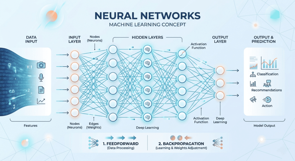
Consider the problem of recognising a handwritten digit. A single neuron can’t do it — there’s no linear combination of pixel values that reliably separates a 3 from an 8. But a network with a hidden layer in the middle can. The first layer of neurons each respond to small, local patterns in the pixels. The second layer combines those responses into higher-level patterns. By the time information reaches the output layer, the network has built up a complex, non-linear representation of the input.

This is the core of what deep learning actually means. It’s not “more powerful” in an abstract sense. It’s that depth enables hierarchical representation. The first layer learns low-level features. Deeper layers combine those into progressively more abstract concepts — the same way a circuit that computes multiplication doesn’t do it in a single gate, it builds it from sub-circuits for addition, which are built from sub-circuits for bit operations. Depth is the mechanism for compositional reasoning.

Research on circuit complexity shows this mathematically: some functions require exponentially more computing elements in shallow circuits than deep ones. The same principle applies to neural networks. A two-layer network can approximate anything, in theory — but in practice it might need an astronomically wide hidden layer to do it. Depth is often the more efficient solution.

The Forward Pass: Data Flowing Through the Network

Training starts with the forward pass: feed input data into the first layer, let each neuron compute its activation, pass those activations to the next layer, repeat until you reach the output.

def forward_pass(X, weights_list, biases_list):
    activation = X
    for W, b in zip(weights_list, biases_list):
        z = np.dot(activation, W) + b
        activation = sigmoid(z)
    return activation

# Random initialisation for a 3-layer network (3 inputs → 4 hidden → 2 output)
np.random.seed(42)
W1 = np.random.randn(3, 4) * 0.1
b1 = np.zeros(4)
W2 = np.random.randn(4, 2) * 0.1
b2 = np.zeros(2)

X = np.array([[0.8, 0.3, 0.9]])
prediction = forward_pass(X, [W1, W2], [b1, b2])
print(f"Output: {prediction}")

The first forward pass produces wrong answers. The network has random weights and has learned nothing. What happens next is where the real machinery is.

Backpropagation: The Blame Assignment Problem

Once the forward pass produces a prediction, you compare it to the correct answer using a loss function — a number that measures how wrong the prediction was. The goal of training is to adjust weights so that loss decreases.

But here’s the problem: the network might have millions of weights. How do you know which ones to adjust, and by how much? The answer is backpropagation, and the right way to think about it is as a systematic solution to blame assignment.

When the prediction is wrong, every weight in the network contributed to that error — some a lot, some barely at all. Backpropagation figures out exactly how responsible each weight was for the overall loss. The core quantity it computes, for every single weight in the network, is the partial derivative of the loss with respect to that weight. That derivative tells you: if I nudge this weight slightly, how much does the loss change? A large derivative means this weight has a strong influence on the error and deserves a larger adjustment. A near-zero derivative means this weight barely affected the outcome.

The algorithm works backward through the network — from output to input — because each layer’s blame depends on the blame computed for the layer in front of it. The chain rule from calculus makes this propagation possible: the derivative of a composed function can be broken into the product of the derivatives of each component function. Backpropagation is essentially the chain rule applied systematically to every weight in the network.

This was understood mathematically in the 1970s, but its real impact wasn’t recognized until a 1986 paper by David Rumelhart, Geoffrey Hinton, and Ronald Williams demonstrated that it ran dramatically faster than alternative learning approaches, making neural networks practical on problems that had previously been unsolvable. That paper’s insight was less about the math — the math was known — and more about showing that backpropagation scaled.

The practical mechanics — how gradients flow, how the chain rule is applied layer by layer, and what happens when networks get very deep — are covered in depth in the backpropagation post. But the core intuition is this: backpropagation is not a mysterious optimization trick. It’s a precise accounting of how much blame each weight deserves for the current error.

Why Deep Learning Didn’t Work Until 2012

If backpropagation was known in 1986, and neural networks were understood theoretically, why did it take until the early 2010s for deep learning to dominate?

The answer is a problem that emerges specifically when networks get deep: the vanishing gradient.

During backpropagation, gradients are computed by repeatedly multiplying numbers together as the algorithm moves backward through layers. Each time you pass through a layer with sigmoid activation, the gradient gets multiplied by the derivative of the sigmoid function — which is always between 0 and 0.25. Multiply a number by 0.25 once and it shrinks. Multiply it through 10 layers and it becomes effectively zero.

The practical consequence is that the early layers of a deep network receive near-zero gradient signals during training. Their weights barely update. They don’t learn. The front of the network stays nearly random while only the later layers improve. Deep networks were, in a meaningful sense, too deep to train.

This problem kept the field stuck for over a decade. Three things broke the deadlock. First, ReLU — a simpler activation function that doesn’t squash gradients — replaced sigmoid in deep networks and let gradients flow more cleanly. Second, better weight initialisation schemes stopped gradients from exploding or vanishing at the very start of training. Third, GPUs provided the computational power to train large networks on large datasets, and it turned out that scale helped gradients behave more stably. The famous 2012 AlexNet result — a deep convolutional network that dramatically outperformed other approaches on ImageNet — was the moment these pieces came together publicly.

What This Post Didn’t Cover

This post deliberately stayed at the level of intuition and mechanism. I didn’t go into the mathematics of the chain rule derivation, or how different loss functions affect gradient behavior, or why weight initialisation matters so much in the early stages of training. Those are real and important — but they follow naturally from understanding the framework here.

For a free, rigorous treatment of the full mathematics — one of the best technical explanations of neural networks written for human beings rather than mathematicians — Michael Nielsen’s Neural Networks and Deep Learning is worth your time. It’s free, thorough, and the backpropagation chapter in particular is clearer than most textbooks.

FAQ

The thing I find most interesting about neural networks, even after working with them for a while, is that the intuition holds all the way from a single neuron to systems with hundreds of billions of parameters. The neuron still computes a weighted sum. The network still learns by assigning blame. The depth still encodes hierarchy. What changes is scale — and at scale, hierarchy becomes capable of remarkable things.

What still puzzles me is the generalization question. A network trained on enough text doesn’t just memorize patterns; it appears to develop something that functions like reasoning. Whether that’s genuine reasoning or an extraordinarily elaborate pattern match is a question the field is actively working through. Worth keeping an eye on.