RNNs and LSTMs Explained: How Neural Networks Remember
Think about how you read. When you get to the word “it” in the middle of a paragraph, you don’t process it in isolation. You carry context forward. You remember what “it” refers to because you’ve been accumulating meaning from everything that came before. Every word lands inside a running interpretation built from the whole sequence so far.
Standard neural networks can’t do that. They read one input, produce one output, and move on. Each forward pass is stateless. The network has no memory of what came before, no way to carry meaning across timesteps. That works fine for classifying a single image or predicting a house price from a fixed set of features. It completely breaks down for language, audio, stock prices, sensor readings, or anything where the order and history of inputs actually matters.
Recurrent Neural Networks, and later Long Short-Term Memory networks, were built specifically to solve this. They’re the architectures that gave deep learning its first serious foothold in sequential data. Understanding how they work, and more importantly why they were so hard to train correctly, tells you something important about what deep learning can and can’t do by default.
Table of Contents
What Makes a Neural Network “Recurrent”
The key concept is deceptively simple: the output of the network at one timestep becomes part of the input at the next.
In a standard feedforward network, information flows in one direction only. Input goes in, passes through layers, output comes out. No feedback, no memory. Formally, you can think of a recurrent neural network as a dynamical system — a system where the current state depends on the previous state. Ghojogh & Ghodsi (2023) frame it this way precisely: an RNN is a dynamical system with external input, where the hidden state at time t is a function of both the current input and the previous hidden state.
What the network maintains is called the hidden state. At each timestep, the network computes a new hidden state from two things: the current input, and the hidden state it computed one step earlier. That hidden state is then passed to the output layer and carried forward to the next timestep. It’s the network’s working memory — a compressed representation of everything it’s processed so far.
The math underneath this looks like:
h_t = tanh(W · h_{t-1} + U · x_t + b)
y_t = V · h_t
Where h_t is the hidden state at time t, x_t is the input, and W, U, V are weight matrices the network learns. The tanh squashes the hidden state into the range (-1, 1) at each step.
Here’s what’s actually interesting about this: those weight matrices W, U, and V are shared across every single timestep. The same parameters handle position 1, position 50, and position 1000 of any sequence. This isn’t a coincidence or a shortcut — it’s the architectural decision that allows an RNN to generalize to sequences of any length. If the network used different weights for each position, it would have no way to apply what it learned at one position to another. Shared parameters are what make sequence modeling possible in the first place.
The Training Problem Nobody Warned You About
Here’s where things get difficult. Training an RNN means training it across time, which is done via an algorithm called Backpropagation Through Time (BPTT). The idea is that you unroll the network across all T timesteps, treat it like a very deep feedforward network, and compute gradients using the chain rule — but now the chain rule also runs backward through time.
Bengio and colleagues formally described the consequence of this in 1993 and 1994: the vanishing gradient problem.
To understand it, you need to think about what happens when you multiply the same matrix repeatedly. The gradient flowing back from timestep T to some earlier timestep t involves multiplying a Jacobian matrix many times in sequence — once per timestep between t and T. That Jacobian matrix is approximately W scaled by a factor that depends on the current hidden state.
If the eigenvalues of that matrix are less than 1, repeated multiplication drives the product toward zero. The gradient vanishes. By the time it reaches the early timesteps, it’s so small that those early weights receive essentially no learning signal. The network can’t learn that something that happened far back in the sequence is relevant to what’s happening now.
This is the concrete mechanism behind something you’ll hear described vaguely as “RNNs forget.” They don’t forget in some fuzzy metaphorical sense — the gradient literally cannot propagate back far enough to update the weights that encoded early context. The network learns short-term dependencies reasonably well. Long-term dependencies effectively become inaccessible.
To make this concrete: consider two sentences. In “The police is chasing the thief,” the words “police” and “thief” are close together — short-term dependency. In “I was born in France… that is why I speak French,” the connection between “France” and “French” is separated by many words — a long-term dependency. A standard RNN can learn the first kind of relationship. The vanishing gradient problem makes the second kind extremely difficult to learn reliably (Ghojogh & Ghodsi, 2023).
The same problem appears in reverse as gradient explosion, when those eigenvalues are greater than 1 and repeated multiplication sends gradients to infinity. That one’s actually easier to fix — you clip the gradients. Vanishing gradients are the harder problem.
What LSTM Actually Fixed
Hochreiter and Schmidhuber introduced the Long Short-Term Memory network in 1997 to handle exactly this. The solution isn’t to change the training algorithm — it’s to change the architecture so that the gradient has a path to flow through time without being repeatedly multiplied through squashing functions.
The key innovation is the cell state: a separate memory track that runs alongside the hidden state, connected to the rest of the network only through three learned gating mechanisms. Unlike the hidden state which gets squashed through tanh at every step, the cell state can carry information forward across many timesteps with minimal modification. Gradients flowing backward through the cell state encounter addition rather than repeated multiplication, which is what prevents them from vanishing.
The three gates each have a specific job:
The forget gate takes the current input and the previous hidden state, runs them through a sigmoid function, and produces a number between 0 and 1 for each element of the cell state. Multiply by 0 and you erase that element. Multiply by 1 and you keep it perfectly. Everything in between is partial retention. This is where the network learns what to drop from memory.
The input gate works in two parts. One sigmoid decides which parts of the cell state to update. A separate tanh layer produces candidate values for those positions. The two are multiplied together — so the network is simultaneously deciding what to update and what those updates should contain.
The output gate decides what part of the cell state to expose as the hidden state at this timestep. Not everything in the cell state is relevant to every output — the output gate filters it. The cell state passes through tanh (scaling it to (-1, 1)), then gets multiplied by the output gate’s sigmoid to produce the final hidden state.
In code, an LSTM layer in practice looks straightforward even though the internals are doing all of this:
import torch
import torch.nn as nn

# Single-layer LSTM: 10 input features, 64 hidden units
lstm = nn.LSTM(input_size=10, hidden_size=64, batch_first=True)

# Sequence of 32 samples, 50 timesteps, 10 features
x = torch.randn(32, 50, 10)
output, (h_n, c_n) = lstm(x)

# output: (32, 50, 64) — hidden state at every timestep
# h_n:    (1, 32, 64)  — final hidden state
# c_n:    (1, 32, 64)  — final cell state
Notice that the LSTM returns both h_n (the hidden state) and c_n (the cell state) separately. That separation is the whole point. The cell state is the long-term memory; the hidden state is what gets passed to the output layer and the next timestep.
GRU: What Happens When You Simplify LSTM
In 2014, Cho and colleagues proposed the Gated Recurrent Unit, which simplifies the LSTM architecture by merging the forget and input gates into a single update gate, and combining the cell state and hidden state into one. The result is two gates instead of three, fewer parameters, and faster training.
The honest comparison: GRU performs comparably to LSTM on many tasks, particularly with smaller datasets where the reduced parameter count prevents overfitting. LSTM tends to have an edge on tasks with very long sequences or tasks where the separation between short-term and long-term memory is genuinely important. In practice, the difference is often small enough that trying both and comparing validation performance is more useful than reasoning about which should win theoretically.
GRU trains faster. LSTM often generalizes better with more data. Neither universally dominates the other, and Greff et al. (2016) — a comprehensive LSTM variant comparison study — found that none of the architectural variants they tested consistently outperformed vanilla LSTM across all tasks. The architecture matters less than most people assume; the training setup, data quality, and sequence length matter more.
Where RNNs and LSTMs Actually Work
Despite Transformers dominating the conversation since 2017, LSTMs and RNNs haven’t disappeared. Obaido (2024) documents their current active use across: natural language processing tasks where sequence order is critical, speech recognition systems where audio frames arrive as a stream, time series forecasting for sensor data and financial signals, anomaly detection in network traffic, and even autonomous vehicle control systems processing sensor sequences.
The reason they persist in some of these domains is practical: LSTMs process one timestep at a time, which makes them well-suited for streaming applications where you don’t have the full sequence available before you need to make a decision. Transformers require the full sequence upfront — their attention mechanism computes relationships between all positions simultaneously. If you’re doing real-time speech recognition on a device with limited memory, an LSTM is often still the right tool.
Time series forecasting is a case where LSTM remains particularly relevant. A sequence of temperature readings, electricity demand values, or server latency measurements has genuine temporal dependencies — what happened in the last 24 hours affects what happens now. An LSTM can model those dependencies without requiring the full reformulation that a Transformer demands.
# Simple LSTM for time series forecasting
class TimeSeriesLSTM(nn.Module):
    def __init__(self, input_size, hidden_size, output_size):
        super().__init__()
        self.lstm = nn.LSTM(input_size, hidden_size, batch_first=True)
        self.fc   = nn.Linear(hidden_size, output_size)

    def forward(self, x):
        out, _ = self.lstm(x)
        # Take the last timestep's output for prediction
        return self.fc(out[:, -1, :])
Bidirectional LSTMs: What the Research Actually Says
A bidirectional LSTM processes the sequence in both directions — one pass forward through time, one pass backward — then concatenates both hidden states. The intuition is that context from future tokens sometimes matters for understanding the current position. In the sentence “I need to book a ticket to the bank,” whether “bank” means a financial institution or a riverbank depends on context that may come later in the sentence.
What most explanations miss is the constraint that makes this possible: bidirectional processing only works when the full sequence is available before processing begins. Graves and Schmidhuber (2005) — who developed bidirectional LSTM — were explicit about this: the model is suitable for sequences that “can be processed offline.” You can’t use a bidirectional LSTM for streaming audio in real time, because you don’t have the future timesteps yet. That’s not a limitation of the implementation — it’s mathematically unavoidable.
The Attention Mechanism and What Replaced RNNs
LSTM’s dominance ended with the Transformer architecture (Vaswani et al., 2017), which replaced sequential hidden state passing with an attention mechanism that computes relationships between all sequence positions simultaneously. This solved the LSTM’s remaining weakness: even with the cell state, information still had to travel through many timesteps to connect distant positions, and the path could get noisy.
But the story isn’t simply “Transformers won.” As noted in the Springer deep learning textbook by Ghojogh & Ghodsi (2026), the recurrent principle has re-emerged in State Space Models like S4 and Mamba, which compete with Transformers for long-sequence efficiency by combining ideas from dynamical systems theory with selective memory gating. The recurrent structure that defined RNNs turns out to have been solving a real problem — the problem was how it handled gradients, not the fundamental idea of maintaining state across time.
The Transformer architecture post covers how attention mechanisms work and why they eventually displaced sequential processing for most NLP tasks.
FAQ
What is the difference between RNN and LSTM?
A standard recurrent neural network passes a hidden state forward through time, but its training algorithm causes gradients to vanish when sequences are long, making it impossible to learn dependencies that span many timesteps. LSTM adds a separate cell state maintained by three learned gating mechanisms — forget, input, and output gates — that allows gradients to flow backward through time without being repeatedly squashed. The cell state is the architectural innovation; it provides a gradient highway that standard RNNs lack.
When should you use LSTM instead of a Transformer?
Use an LSTM when your task involves streaming data where you need to process inputs one at a time without the full sequence available in advance, when your dataset is small enough that Transformer’s parameter count causes overfitting, or when computational resources are constrained. For offline tasks with large datasets, Transformers generally outperform LSTMs, especially for tasks with very long-range dependencies. The choice is practical, not philosophical.
What is the vanishing gradient problem in recurrent neural networks?
When training an RNN using Backpropagation Through Time, gradients must propagate backward through every timestep. Each step involves multiplying by a Jacobian matrix. If the eigenvalues of that matrix are less than 1, repeated multiplication drives the gradient exponentially toward zero. Weights at early timesteps receive an effectively zero learning signal, so the network can’t learn that early inputs matter to later outputs. LSTM’s cell state avoids this by providing an additive path for gradients rather than a multiplicative one.
There’s something worth sitting with here: the vanishing gradient problem was formally described in 1993. LSTM was the direct response to it in 1997. The gating mechanism isn’t an arbitrary design choice — it’s a mathematically motivated fix to a specific, well-understood failure mode. That’s the pattern you see repeatedly in deep learning: architectures aren’t invented arbitrarily. They’re answers to clearly diagnosed problems, and understanding the diagnosis is what makes the architecture legible.