Bias-Variance Tradeoff: The Concept That Explains Most ML Failures

Think about two different archers.

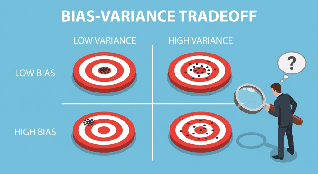
The first one clusters all her arrows in the same spot, but that spot is a foot to the left of the bullseye. Consistent. Wrong. The second one hits all over the target, sometimes close to center, sometimes not, but with no reliable pattern. Inconsistent. Also wrong, just differently.

That’s bias and variance. High bias is the first archer: your model is consistently wrong in the same direction because it’s too simple to capture the real pattern. High variance is the second: your model is erratic because it’s too sensitive to the specific training data it happened to see, and it’d look completely different if you retrained on a slightly different sample.

Both archerss miss. They miss for opposite reasons. And almost every model failure you’ll encounter is some version of one of these two problems.

The bias-variance tradeoff is the formal way of thinking about this, and once it clicks, you’ll start diagnosing model problems faster. Not because it gives you a formula, but because it forces you to ask the right question: is my model failing because it’s too simple, or because it’s too sensitive?

The Math, Briefly

You don’t need to derive this, but seeing the decomposition once is useful.

The expected prediction error of a model on a new data point can be broken into three parts:

Total Error = Bias² + Variance + Irreducible Noise

Bias is the error from wrong assumptions. It’s the gap between what your model predicts on average across many training runs and what the true answer actually is.

Variance is the error from sensitivity to training data. It measures how much your model’s predictions would change if you trained it on a different sample from the same distribution.

Irreducible noise is the floor. It’s the error that exists in the data itself, measurement error, randomness, factors you didn’t capture. No model eliminates this. It’s called irreducible because it is.

The tradeoff exists because the things you do to reduce bias tend to increase variance, and vice versa. Adding model complexity reduces bias but inflates variance. Adding regularization reduces variance but introduces bias. You’re moving weight between two buckets, and the floor is always there.

High Bias: When Your Model Is Too Sure of the Wrong Thing

A high-bias model has made strong assumptions that are wrong.

The classic example is fitting a straight line to data that follows a curve. Linear regression assumes the relationship is, well, linear. If it isn’t, the model will be consistently wrong in a predictable way across the whole dataset. Training error will be high. Test error will also be high, and roughly equal to training error. That’s the signature of underfitting: both errors are bad and they’re close together.

In practice, you see high bias when you’re using a model that’s too simple for the task. Logistic regression on a problem that needs a decision boundary that isn’t a line. A shallow decision tree on data with complex interactions. A linear model on image data.

The fix is more model complexity, better features, or both. You need to give the model more capacity to represent the actual relationship in the data.

But here’s the thing worth saying plainly: high bias is underdiagnosed. People reach for complex models by default in 2026 because complex models are easy to spin up with modern libraries. So they rarely hit the high-bias ceiling. But when they do, adding data doesn’t help much because the model can’t use it. It’s already capped by its own structural limitations.

High Variance: When Your Model Knows Too Much About One Dataset

A high-variance model has memorized rather than learned.

Training error is low. Test error is significantly higher. That gap, which I cover in more detail in the overfitting post, is the fingerprint. If you retrained the same model on a different random sample from the same population, you’d get substantially different predictions. The model is following the noise.

High variance usually comes from too much model complexity relative to the amount of data. A deep neural network trained on 500 examples. A decision tree with no depth limit. A polynomial regression of degree 15 on a dataset where the true relationship is degree 2.

You can also get high variance from noisy features. If you’re feeding irrelevant or noisy inputs to a flexible model, it’ll find patterns in those inputs because it’s trying hard to minimize training error. Those patterns don’t exist in the real world.

The fixes are what you’d expect: more data, simpler model, regularization. Getting more data is often the most reliable fix, but the least convenient one.

The Tradeoff: Why You Can’t Just Fix Both

This is the part that trips people up.

You’d think you could just tune bias and variance independently. Fix the bias by adding complexity, then fix the variance by adding regularization. In practice, they push against each other because they’re both responding to the same thing: how much structure you’re imposing on what the model can learn.

Adding a regularization term to penalize large weights reduces variance (the model becomes less sensitive to individual training points) but introduces bias (you’re constraining the model’s ability to fit the true function). Removing regularization reduces bias but allows variance to climb.

As model complexity increases, bias goes down and variance goes up. There’s a sweet spot somewhere in between where total error is minimized. That’s the U-curve you’ll see in every textbook diagram of this concept. The left side of the curve is underfitting territory, high bias, and the right side is overfitting territory, high variance.

Model selection is fundamentally the exercise of finding where you are on that curve and deciding which direction to move. Every time you’re choosing between a simpler and more complex model, you’re making a bias-variance decision, whether you frame it that way or not.

How Model Complexity Moves the Dial

Let me make this concrete with decision trees, because the complexity knob is visible and easy to reason about.

from sklearn.tree import DecisionTreeClassifier from sklearn.model_selection import train_test_split from sklearn.metrics import accuracy_score X_train, X_test, y_train, y_test = train_test_split(X, y, test_size=0.2, random_state=42) for depth in [2, 4, 8, 16, None]: clf = DecisionTreeClassifier(max_depth=depth, random_state=42) clf.fit(X_train, y_train) train_acc = accuracy_score(y_train, clf.predict(X_train)) test_acc = accuracy_score(y_test, clf.predict(X_test)) print(f”depth={str(depth):4s} train={train_acc:.3f} test={test_acc:.3f} gap={train_acc – test_acc:.3f}”)

Run this on a real dataset and you’ll typically see something like:

• depth=2: both scores low, small gap (high bias, underfitting)
• depth=4: both scores decent, small gap (reasonable fit)
• depth=8: training climbs, test climbs less, gap growing
• depth=None: training near-perfect, test significantly lower (high variance, overfitting)

The sweet spot is wherever test accuracy peaks. That’s your model complexity optimum for this dataset and split. Watching that gap across complexity levels is one of the more reliable tools I use for model selection in practice, and it connects directly to what cross-validation formalizes in the cross-validation post.

What Actually Reduces Variance Without Killing Bias

This is where ensemble methods earn their reputation.

Bagging (bootstrap aggregating) trains many versions of the same model on different random subsets of the training data, then averages their predictions. The averaging step is the key move. When you average many high-variance models, the noise in each prediction is uncorrelated across models, so it tends to cancel out. What’s left is the signal they all agreed on.

Random forests are the canonical example. Each tree is a high-variance model on its own. But averaged across 100 or 500 trees trained on different bootstrapped samples with different random feature subsets, the ensemble has dramatically lower variance than any individual tree, and bias stays roughly the same or even improves slightly.

Boosting works differently. It reduces bias by building models sequentially, where each new model corrects the errors of the previous one. But it can increase variance if you push it too far, which is why early stopping and learning rate control matter so much with gradient boosting.

I once spent an afternoon trying to tune a single deep decision tree to match the performance of a 100-tree random forest. It never got there. The ensemble wasn’t just “more trees,” it was exploiting variance reduction in a way a single model structurally can’t. That was an expensive lesson in understanding why the tools work, not just that they work.

The Part Nobody Tells You About Modern ML

Here’s something that’s worth being honest about: the classical bias-variance tradeoff picture doesn’t fully explain what happens with modern deep learning.

The U-curve says that past a certain complexity, test error should climb as variance dominates. But large neural networks often don’t follow this. They can be massively overparameterized (far more parameters than training examples) and still generalize surprisingly well. Researchers have found that if you keep increasing model size past the classical overfitting peak, test error sometimes comes back down again. This is called double descent, and I genuinely don’t have a fully satisfying intuition for why it happens. The theoretical understanding is still catching up to the empirical observation.

What this means practically: the tradeoff framework is extremely useful for traditional ML (tree-based models, linear models, SVMs) and for smaller neural networks. For large foundation models, the rules are different in ways that aren’t fully understood yet. Don’t throw out the framework, but hold it a bit more loosely when you’re working at scale.

What This Post Didn’t Cover

The formal derivation of the bias-variance decomposition from expected squared error. It’s worth doing once if you want to feel the math, but it doesn’t change how you use the concept.

I also didn’t go into per-algorithm bias-variance profiles in depth. Linear models have high bias by design. KNN has low bias but high variance (especially at small k). Naive Bayes has high bias from its independence assumption but often surprisingly low variance. Each algorithm has a characteristic position on the tradeoff that’s worth understanding separately.

FAQ

---

The bias-variance tradeoff doesn’t tell you exactly where to set your regularization strength. That’s a question for cross-validation and domain knowledge. What it does tell you is the direction of the error you’re introducing and what to watch for when you’ve pushed too far in either direction.