How Machine Learning Works: A Step-by-Step Breakdown

You upload 10,000 photos of cats and dogs, press train, wait 20 minutes, and now your model can tell them apart.
But what actually happened during those 20 minutes? Something did. The model went from knowing nothing to being right 94% of the time. That change didn’t happen by accident, and it wasn’t magic. There’s a specific mechanical process running in that loop, and once you see it clearly, the whole field becomes much less mysterious.
This is what machine learning actually does, step by step.
Table of Contents
The Setup: What Goes In
Before training starts, three things have to exist: data, a model architecture, and a task definition.
Definition: Machine learning is the process of adjusting a model’s internal parameters (weights) so that its predictions improve on a training dataset. The model learns by measuring its own errors and making small corrections repeatedly until the errors get small enough to be useful.
The data pipeline is the first place things go wrong in practice, and it’s the part tutorials skip over fastest. Your raw data, whatever form it’s in, needs to reach the model in a format it can process. For images, that means pixel values. For text, that means token indices. For tabular data, that means numerical columns with missing values handled and categorical columns encoded.
Getting the data pipeline right sounds boring. It isn’t. In production, data pipeline issues cause more model failures than model issues do. But that’s a separate post.
What you also need before training: a split. You set aside a portion of your data as a validation set that the model never trains on. Typically 80% trains, 20% validates. This held-out chunk is what lets you check whether learning is actually happening, and it’s what catches overfitting before it embarrasses you in production. I’ve written about that failure mode in detail in the overfitting post, but the short version is: if you don’t hold data out, you have no way to know if your model learned the task or just memorized your training examples.
The Training Loop: What Actually Runs
The training loop is the core of machine learning. Everything else is setup or cleanup. The loop itself is four steps, repeated thousands of times.
Step 1: Forward pass. The model takes one batch of training examples, runs them through its current parameters, and produces predictions. At the start of training, these predictions are essentially random. That’s fine.
Step 2: Measure the error. The predictions get compared to the correct answers using a loss function. The loss function returns a single number that represents how wrong the model is right now. High loss means bad predictions. Zero loss would mean perfect predictions (and would also probably mean something is wrong).
Step 3: Backward pass. The model figures out which parameters were responsible for the error, and by how much. This step uses calculus: specifically the chain rule. Each parameter gets assigned a gradient, which tells you whether increasing or decreasing that parameter would reduce the loss, and roughly by how much.
Step 4: Update. Gradient descent uses those gradients to nudge every parameter in the direction that reduces loss. The size of the nudge is controlled by the learning rate. Small learning rate means slow, stable learning. Large learning rate means faster but riskier updates that can overshoot.
Then the loop repeats.
One pass through all your training data is an epoch. Most models train for tens or hundreds of epochs. By the end, the parameters have been adjusted thousands or millions of times, all in the direction of lower loss.
Loss Functions: Measuring How Wrong You Are
The loss function deserves its own section because people treat it like a formality when it’s actually a design decision that shapes what your model optimizes for.
For regression, mean squared error is the default. It penalizes large errors more than small ones because squaring amplifies them. If you care about outliers, that’s a feature. If outliers are noise you don’t care about, it’s a problem.
For classification, cross-entropy loss is standard. It measures how far your predicted probability distribution is from the true label distribution. A model that says “70% cat, 30% dog” when the answer is dog gets penalized less than one that says “95% cat, 5% dog.”
The practical thing to understand: your model will optimize exactly what you tell it to, nothing more. If your loss function doesn’t capture what you actually care about, the model will find ways to score well on the loss while failing on the thing you actually wanted. This happens constantly in practice, and it’s one of the rougher edges of the field.
Gradient Descent: The Correction Mechanism
Weights are the learnable parameters inside a model. In a simple linear model, you have a weight for each input feature. In a neural network with millions of parameters, you have weights inside every layer. They all start at some initial value (often random, sometimes informed) and the training loop adjusts them.
Gradient descent is the adjustment mechanism. The gradient tells you the slope of the loss function with respect to each weight: if you increase this weight, does loss go up or down, and by how much? Gradient descent moves each weight a small step in the direction that reduces loss.
The mountain-climbing analogy is overused but accurate: imagine you’re on a foggy hillside and want to reach the lowest point. You can’t see the full landscape. But you can feel which direction is downhill from where you’re standing. So you take a step downhill, look around, take another step downhill, and repeat. Gradient descent is that process, but in a space with millions of dimensions.
A few things make this messy in practice. The loss landscape isn’t smooth. There are local minima you can get stuck in, saddle points that look like minima but aren’t, and flat regions where gradients are near zero and learning stalls. Modern optimizers like Adam handle most of these by adapting the learning rate per parameter, which is why most practitioners use Adam by default rather than vanilla gradient descent.
The Validation Set: Catching Problems Early
While the training loop runs, you periodically pause and check performance on the validation set. The model doesn’t train on this data. You just run predictions through it and check the loss.
What you’re watching for is the relationship between training loss and validation loss over time. Both should decrease as training progresses. If training loss keeps dropping but validation loss starts rising, the model is beginning to memorize training data instead of learning generalizable patterns. That’s the overfitting signal, and early stopping uses it to halt training before the problem gets worse.
The validation set is also where you make decisions about hyperparameters. Which learning rate? How many layers? How much regularization? You try variations, compare validation performance, and pick the version that performs best on held-out data.
Here’s something that catches beginners: once you’ve used a validation set to make enough decisions, it’s no longer truly independent. You’ve leaked information from it into your model selection process. This is why serious evaluation uses a separate test set that you look at exactly once, at the very end. The validation set is for experimentation. The test set is for the final honest report card. I go into the mechanics of this further in the post on train, validation, and test splits, which covers how to get the split right without accidentally leaking data between sets.
Inference: Using What the Model Learned
After training, you freeze the weights and stop updating them. What you have is a fixed function that maps inputs to predictions. Running that function on new data is called inference.
Inference is computationally cheaper than training because there’s no backward pass, no gradient calculation, no weight updates. You’re just running the forward pass and reading the output.
But inference is where the model has to actually work, and it’s where a lot of assumptions get tested. The training data and the inference data need to come from the same distribution. If you train on cats and dogs photographed on white backgrounds and then run inference on blurry outdoor photos, performance will drop. Not because the model is broken, but because you’re asking it to generalize beyond what it saw.
This distribution shift problem is, honestly, one of the most persistent and underappreciated issues in production ML. Models work in the lab and fail in the real world not because the algorithm is wrong but because the real world doesn’t look like the training data.
The Part Nobody Warns You About
Here’s the thing nobody tells you when you first learn this step-by-step picture: the loop is messier than it looks.
The neat four-step narrative implies a smooth process where loss steadily decreases and you watch it converge to a good solution. Real training isn’t like that. Loss curves spike. Validation performance plateaus for 10 epochs and then suddenly improves. The model behaves differently depending on batch size, initialization seed, and data ordering. Two runs of the exact same code don’t always produce the same result.
What you’re actually doing when you train a model is running a complicated optimization process on a non-convex landscape with noisy gradients, and watching the metrics to guess whether it’s going somewhere useful. Experience teaches you to read the signals. But I don’t want to pretend it’s as tidy as the step-by-step framing makes it sound.
Also worth naming: the data pipeline is genuinely half the job. The training loop gets all the attention because it’s where the math lives. But in practice, you’ll spend more time cleaning data, handling missing values, debugging transform errors, and investigating why your batches look wrong than you’ll spend thinking about gradient descent.
What This Post Didn’t Cover
I kept this post at the conceptual level and skipped the math. Specifically, I didn’t derive the backpropagation algorithm or show how gradients actually get computed through a network. That deserves its own post and a lot more space than I have here.
I also didn’t get into specific optimizers (Adam, RMSprop, SGD with momentum) or learning rate schedules, both of which matter a lot in practice. Those are implementation details that build on this foundation rather than changing the core picture.
FAQ
How long does training a machine learning model take?
It depends entirely on the model size, dataset size, and hardware. A small sklearn model on tabular data trains in seconds. A fine-tuned transformer on a GPU takes hours. Large language models trained from scratch take months on thousands of specialized chips. For most practical projects you’re starting out on, training time is measured in minutes to hours.
What’s the difference between training and inference in machine learning?
Training is the process of adjusting the model’s weights by running the training loop repeatedly over labeled data. Inference is using the trained, frozen model to make predictions on new data. Training is compute-heavy and happens once (or periodically). Inference is lighter and happens continuously in production.
Why does my model’s training loss decrease but validation loss doesn’t?
This is the classic overfitting signal. Your model is learning to perform well on the training examples specifically, rather than learning patterns that generalize. The fixes in rough order of what to try: more training data, a simpler model architecture, regularization (dropout, L1/L2), or early stopping. Check your data for leakage or duplicates first before assuming it’s a model complexity problem.
The step-by-step framing in this post makes the process look more sequential and controllable than it is. But the underlying mechanics are real, and understanding them pays off. Once you know what a loss function is doing and why gradient descent moves in the direction it does, debugging a training run stops feeling like guesswork.
What I’m still watching carefully: alternative training paradigms that don’t use gradient descent at all. Evolutionary methods, second-order optimizers, and some newer approaches to training large models suggest the four-step loop might not be the only story for long. The fundamentals here will stay relevant, but the implementation might look different in a few years.