K Nearest Neighbors Algorithm: How It Works and Why It Fails

Most algorithm posts will tell you KNN is a beginner algorithm, a stepping stone before you get to “real” methods. That framing is wrong, and it sends people in the wrong direction.

Cover and Hart proved in 1967 that the nearest neighbor rule, at its simplest with k=1, achieves an error rate bounded above by twice the theoretically optimal error rate, what statisticians call the Bayes error. That bound holds regardless of the underlying data distribution. No assumptions required. No parameters to fit. Just distances and a vote. For a method that requires no training computation at all, that’s a remarkable theoretical guarantee, and it’s why KNN still appears in production systems across recommendation engines, anomaly detection, and medical diagnostics in 2026.

The algorithm’s actual problem isn’t simplicity. It’s that most people misunderstand what drives its performance, and as a result they misuse it in ways that quietly destroy the very property that makes it powerful.

What the Algorithm Actually Does

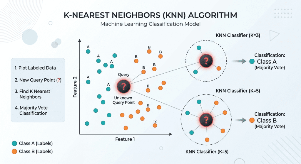
The k-nearest neighbors algorithm classifies a new data point by finding the k most similar points in the training set and taking a majority vote on their labels. For regression it takes the average of their values instead. Nothing is learned ahead of time. No model is fitted. The training data is the model.

Definition: KNN is a nonparametric, instance-based supervised learning algorithm. During prediction, it computes the distance between an incoming data point and every point in the training set, retrieves the k nearest neighbors, and assigns the majority class (for classification) or the mean value (for regression) of those neighbors as the output. Because all computation happens at prediction time rather than training time, it is classified as a lazy learning algorithm.

The term lazy learning isn’t a criticism. It describes a precise technical property: the algorithm defers all generalization to query time rather than building an explicit model during training. The cost is paid at inference, not upfront. This is actually a genuine advantage in some settings. When your data distribution shifts over time, KNN adapts automatically because you can simply add new training points and the model updates instantly. There’s no retraining step.

from sklearn.neighbors import KNeighborsClassifier
from sklearn.preprocessing import StandardScaler
from sklearn.model_selection import train_test_split
from sklearn.metrics import accuracy_score

X_train, X_test, y_train, y_test = train_test_split(X, y, test_size=0.2, random_state=42)

scaler = StandardScaler()
X_train_scaled = scaler.fit_transform(X_train)
X_test_scaled  = scaler.transform(X_test)

knn = KNeighborsClassifier(n_neighbors=7, metric='euclidean')
knn.fit(X_train_scaled, y_train)

print(f"Accuracy: {accuracy_score(y_test, knn.predict(X_test_scaled)):.3f}")

Notice the StandardScaler call before fitting. That’s not optional, and I’ll explain exactly why shortly.

The Distance Metric Is Doing Most of the Work

KNN’s entire decision logic rests on one question: what does “nearest” mean? The answer is determined by the distance metric, and the choice matters more than most introductions suggest.

Euclidean distance is the default and the most common. It measures the straight-line distance between two points in feature space. Geometrically familiar, computationally straightforward, and it works well when features are on comparable scales and the underlying relationships in the data are roughly isotropic, meaning direction doesn’t disproportionately favor any feature.

Manhattan distance (also called L1 distance) sums the absolute differences across features rather than squaring them. Research comparing distance metrics across multiple benchmark datasets consistently finds that Manhattan and Euclidean perform comparably for most classification problems, with Euclidean edges slightly ahead on continuous-feature datasets. Manhattan becomes preferable when features are sparse or when the data has outliers, because squaring amplifies the influence of extreme values and Manhattan is more robust to that.

Minkowski distance generalizes both: when the parameter p equals 2 you get Euclidean, when p equals 1 you get Manhattan. Adjusting p lets you tune sensitivity to feature differences.

The practical implication is this: most of the time Euclidean or Manhattan will perform similarly. But the distance metric interacts with feature scale in a way that can completely override any signal the algorithm is trying to detect.

Why Normalization Is Non-Negotiable

KNN computes distances in feature space. If one feature is measured in thousands of dollars and another is measured as a 0-to-1 probability, the dollar-scale feature will dominate every distance calculation. The probability feature becomes invisible. The model will effectively classify based on the single large-scale feature, regardless of what k is set to.

Normalization before KNN is not optional. It’s part of the algorithm. Without it, you’re not running the model you think you’re running.

StandardScaler centers each feature to zero mean and scales to unit variance. MinMaxScaler scales to a fixed range. Either works. The key is that the scaler is fitted on training data only and applied to test data separately, a topic covered in more depth in the feature engineering post, where preprocessing pipelines and why they break when fit on the full dataset are discussed.

Choosing k: The Tension Between Noise and Bias

The k value controls the smoothness of the decision boundary. Small k means the model trusts individual training points closely. Large k means it takes a wider vote and smooths out local irregularities.

k=1 memorizes the training set perfectly. Every training point is its own nearest neighbor, so training accuracy is 100% regardless of your actual data. Cover and Hart’s theoretical guarantee applies asymptotically, meaning with infinite data. In finite samples, k=1 overfits badly.

k=N (all training points) just predicts the majority class every time. No discrimination at all.

The right k lives somewhere between those extremes, and finding it is an empirical question. Cross-validation across a range of k values is the standard approach. Odd values of k are preferred for binary classification because they prevent tie votes. Research on k-value behavior shows that k=2 produces notably worse performance than k=1 or k=3 in binary problems precisely because of the tie-breaking problem: two neighbors in two different classes produces an ambiguous vote.

from sklearn.model_selection import cross_val_score
import numpy as np

k_range = range(1, 31)
scores = []

for k in k_range:
    knn = KNeighborsClassifier(n_neighbors=k)
    cv_scores = cross_val_score(knn, X_train_scaled, y_train, cv=5, scoring='accuracy')
    scores.append(cv_scores.mean())

best_k = k_range[np.argmax(scores)]
print(f"Best k: {best_k}, CV Accuracy: {max(scores):.3f}")

In practice, k values between 3 and 15 cover the majority of well-performing configurations for small-to-medium datasets.

The Curse of Dimensionality: Why KNN Breaks in High Dimensions

This is the failure mode that most tutorials either skip or treat as a footnote. It isn’t a footnote.

The foundational intuition behind KNN is that nearby points in feature space should have similar labels. That intuition relies on distances being meaningful: some points are genuinely close, others are genuinely far, and that contrast is what the algorithm exploits.

In high-dimensional spaces, that contrast collapses.

Research published at ICML 2009 (Radovanović, Nanopoulos, and Ivanovic) demonstrated that as dimensionality increases, a phenomenon called distance concentration emerges: pairwise distances between all data points converge toward the same value. The ratio between the maximum and minimum distances across your dataset approaches 1 as dimensions grow. When everything is approximately equidistant, the concept of a “nearest neighbor” becomes mathematically incoherent.

The same research identified a related and less-discussed phenomenon called hubness. In high-dimensional data, the k-occurrence distribution becomes strongly skewed. Certain data points begin appearing in the k-nearest-neighbor lists of disproportionately many other points. These “hub” points end up mediating a large fraction of all neighbor relationships, and they tend to cluster near the mean of the data distribution rather than being meaningfully representative of the local structure around any query point. The consequence is systematic classification bias that gets worse as dimensionality increases, independent of which distance metric you use.

More recent theoretical analysis (Peng, Gui, and Wu, arXiv 2401.00422, 2025) confirmed these findings using formal proofs: as dimensionality grows, nearest neighbor search using Minkowski distance, Chebyshev distance, and cosine distance all degrade toward meaninglessness. There is no distance metric that fully escapes this.

This is why KNN behaves well on image pixel data or tabular datasets with 10-30 features and often falls apart on text features (thousands of dimensions) or raw genomics data (tens of thousands of dimensions) without aggressive dimensionality reduction first.

The practical rule of thumb: if your feature space has more than 20-30 dimensions and most of those features actually carry signal, apply PCA or another dimensionality reduction step before running KNN. The k-means clustering post covers a related version of this problem, where high-dimensional spaces cause cluster quality to degrade for the same underlying reason.

KNN for Regression, Not Just Classification

KNN works for regression too, and it’s underused in that context. Instead of majority voting, it averages the target values of the k nearest neighbors.

from sklearn.neighbors import KNeighborsRegressor

knn_reg = KNeighborsRegressor(n_neighbors=5, metric='euclidean', weights='distance')
knn_reg.fit(X_train_scaled, y_train)
predictions = knn_reg.predict(X_test_scaled)

The weights='distance' parameter gives closer neighbors more influence on the prediction, which often improves accuracy by reducing the blurring effect of distant neighbors that are technically within the k boundary but not genuinely informative.

KNN regression is particularly useful when the relationship between features and the target is locally smooth but globally complex, situations where linear regression fails because the global relationship isn’t linear, but a flexible model like a neural network would overfit on limited data. It sits in a useful middle ground.

When to Use KNN and When to Walk Away

KNN is a reasonable first choice when your dataset has fewer than a few thousand training examples, features are on a reasonable scale (or can be normalized), the number of features is manageable (under ~30), and interpretability of individual predictions matters. Explaining that a prediction was made because the three most similar historical cases all produced outcome X is genuinely understandable to non-technical stakeholders.

Walk away from KNN when your dataset is large. Prediction time scales with the number of training examples because every query requires computing distance to every stored point. Scikit-learn’s default KNN uses a KD-tree or ball-tree structure that speeds this up, but even with those optimizations, KNN on a million-point training set is slow at inference in ways that rule it out for real-time applications. The scikit-learn KNeighborsClassifier documentation covers the algorithm choices (brute force, KD-tree, ball-tree) and when each makes sense.

Also walk away when your features are high-dimensional without a clear path to dimensionality reduction. The hubness and distance concentration effects aren’t theoretical concerns you can engineer around. They’re mathematical properties of high-dimensional spaces that no distance metric fully escapes.

FAQ