Decision Tree Algorithm: How It Works and Where It Breaks

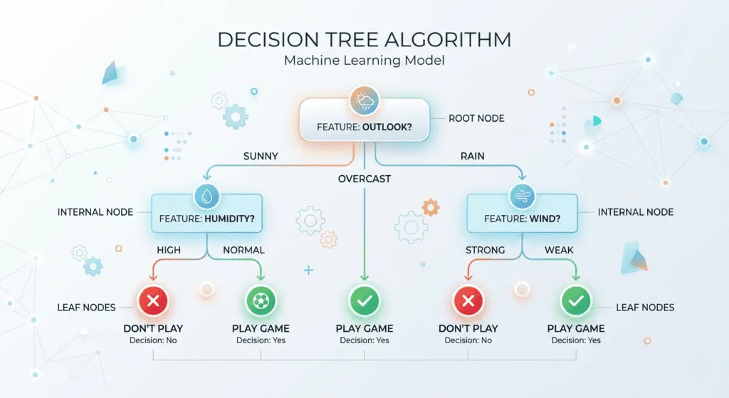
Imagine you’re trying to figure out if a restaurant is worth visiting. You don’t sit down and run a weighted scoring model in your head. You ask a series of questions. Is it too expensive? If yes, skip it. Is the cuisine something you like? If yes, what are the reviews like? If reviews are good and it’s within budget, you go. If not, you don’t.

That’s a decision tree. A series of binary questions, each one narrowing down the answer, until you land on a prediction. The algorithm does exactly this, but it learns which questions to ask, and in what order, directly from your data.

Decision trees are one of the most studied algorithms in the entire history of machine learning. Loh’s 2014 survey in the International Statistical Review traces the lineage back to 1963, sixty-plus years of research across statistics and computer science converging on what is now a standard tool in almost every practitioner’s toolkit. And yet, most explanations of how they work either stop at the analogy or gloss over the parts where they actually break down.

So here’s the full picture: how decision trees learn to split, what the research actually says about Gini versus entropy, and the two failure modes that will bite you in production if you’re not watching for them.

What a Decision Tree Is Actually Doing

At its core, a decision tree algorithm recursively partitions your feature space. Starting from all your training data at the root, it finds the single best split on a single feature, divides the data into two groups, and then repeats the same process on each group independently. It keeps splitting until it hits a stopping condition, which we’ll get to.

Definition: A decision tree is a supervised learning algorithm that makes predictions by learning a series of binary decision rules from training data. At each node, the algorithm selects a feature and a threshold that best separates the data by class or target value. The result is a hierarchical structure that routes new examples to a prediction through a sequence of if-then tests.

The key decision at every node is: which feature to split on, and where. That decision is made by evaluating every possible split across every feature, and choosing the one that creates the most homogeneous subgroups. The mathematical measure of “homogeneous” is what the splitting criterion defines.

Gini Impurity vs Entropy: What Research Actually Found

This is where every tutorial gives you two formulas and then says “both work fine, just pick one.” That’s true but incomplete, and it skips the more interesting finding.

Gini impurity measures how often a randomly chosen element from a node would be misclassified if labeled randomly according to the class distribution in that node. A node containing only one class has Gini of zero (perfectly pure). A node split 50/50 between two classes has Gini of 0.5.

Entropy (used to compute information gain) comes from information theory. A node with one class has entropy of zero. Maximum entropy for a two-class problem is 1. The algorithm picks splits that reduce entropy the most, which is what “information gain” means: the reduction in entropy achieved by that split.

Numerically, the two measures track each other closely. They’re both minimized when a node is pure and maximized when classes are evenly mixed.

Here’s the thing nobody tells you: a 2020 empirical study by Tangirala published in the International Journal of Advanced Computer Science and Applications tested Gini and entropy across balanced and imbalanced datasets and found that “regardless of whether the dataset is balanced or imbalanced, the classification models built by applying the two different splitting indices give the same accuracy.” The choice of splitting criterion affects the size and shape of the tree, but not predictive accuracy in any consistent way.

Earlier empirical work cited in that study found the same result: “choice of the feature selection measure affects the size of the tree but not its accuracy.”

So the question “should I use Gini or entropy?” is mostly a red herring. Gini is cheaper to compute because it avoids logarithms. Entropy can handle imbalanced datasets slightly more gracefully because it penalizes small impurities more heavily. But in production, either gives you a model of equivalent quality.

from sklearn.tree import DecisionTreeClassifier

# Gini (default) — faster, same accuracy
clf_gini = DecisionTreeClassifier(criterion="gini", max_depth=5, random_state=42)

# Entropy — slightly different tree shape, same accuracy
clf_entropy = DecisionTreeClassifier(criterion="entropy", max_depth=5, random_state=42)

clf_gini.fit(X_train, y_train)
clf_entropy.fit(X_train, y_train)

print(f"Gini test accuracy:   {clf_gini.score(X_test, y_test):.4f}")
print(f"Entropy test accuracy: {clf_entropy.score(X_test, y_test):.4f}")
# These will be extremely close, sometimes identical

The scikit-learn DecisionTreeClassifier documentation lists both options and notes that results are “often very similar.” Research has confirmed this empirically at scale.

The Real Innovation in CART (That Most Tutorials Skip)

Breiman, Friedman, Olshen, and Stone published the CART (Classification and Regression Trees) algorithm in 1984, and it transformed the field. But Loh’s 50-year survey makes an important point: the key innovation wasn’t the Gini impurity criterion. Earlier algorithms already had splitting criteria.

What CART introduced that actually mattered was cost-complexity pruning.

Before CART, algorithms like AID and THAID used stopping rules: they stopped splitting when the improvement fell below a threshold. The problem, as Einhorn (1972) had shown by simulation, was that these stopping rules caused overfitting when set too loosely and underfitting when set too tightly. You couldn’t win.

CART’s solution was elegant. Grow the tree as large as possible first, then prune it back using cross-validation to find the size that minimizes generalization error. The pruning procedure works by indexed cost-complexity: you penalize tree complexity and find the “weakest links,” branches that contribute little to performance relative to the complexity they add, and remove them.

This is why pruning is not optional hygiene. It’s the mechanism CART was actually built around. An unpruned decision tree trained to full depth will memorize your training data. Completely. It will hit 100% training accuracy on almost any dataset, because with enough depth there’s always a sequence of splits that partitions your training examples into pure leaf nodes.

That’s not learning. That’s overfitting that happens to look impressive on training metrics.

from sklearn.tree import DecisionTreeClassifier
from sklearn.model_selection import cross_val_score

# Full depth — guaranteed to overfit on small/medium datasets
clf_full = DecisionTreeClassifier(random_state=42)  # no max_depth = unlimited
clf_full.fit(X_train, y_train)

print(f"Train accuracy (full depth): {clf_full.score(X_train, y_train):.4f}")  # will be 1.0
print(f"Test accuracy (full depth):  {clf_full.score(X_test, y_test):.4f}")   # will be much lower

# Post-pruning via cost_complexity_alpha
path = clf_full.cost_complexity_pruning_path(X_train, y_train)
alphas = path.ccp_alphas

# Pick best alpha via cross-validation — this is what CART actually intended
cv_scores = [cross_val_score(DecisionTreeClassifier(ccp_alpha=a, random_state=42),
             X_train, y_train, cv=5).mean() for a in alphas]

best_alpha = alphas[cv_scores.index(max(cv_scores))]
clf_pruned = DecisionTreeClassifier(ccp_alpha=best_alpha, random_state=42)
clf_pruned.fit(X_train, y_train)
print(f"Pruned test accuracy: {clf_pruned.score(X_test, y_test):.4f}")  # usually better

The Failure Mode Nobody Talks About: Variable Selection Bias

Here’s the thing nobody tells you, and it matters if you use feature importance from a decision tree to make any real decision.

Decision trees have a structural bias toward features with many distinct values. The CART algorithm searches over all possible splits on all features greedily. A continuous feature with 1,000 unique values generates 999 candidate split points. A binary categorical feature generates one. All else being equal, the algorithm has far more opportunities to find a “good” split using the high-cardinality feature, even if the binary feature is equally or more predictive.

This bias was acknowledged in the original Breiman et al. (1984) paper itself, and Loh’s survey notes that “White & Liu (1994) and Kononenko (1995) demonstrated its severity in C4.5.” It applies to CART too.

The practical consequence is that feature importance scores from a single decision tree are unreliable when your features have very different cardinalities. A continuous numerical feature will appear more important than a binary categorical feature even when the binary one predicts just as well, simply because of the split-point arithmetic.

This is one of the reasons the random forest approach, which we dig into in detail in the next post, produces better importance scores: by averaging over many trees trained on bootstrap samples with random feature subsets, the cardinality bias gets diluted. A single decision tree doesn’t have that correction.

If you’re using a decision tree’s feature importance to drive any real business decision, check whether your features have similar cardinalities first. If they don’t, treat those scores with caution.

Controlling Depth and When to Stop

Depth is the most direct lever you have over a decision tree’s behavior. A tree with depth 1 makes a single binary decision. A tree with depth 30 can create 2³⁰ leaf nodes, which is more partitions than any reasonable dataset has examples.

Deeper trees have lower bias and higher variance. They fit training data better, including its noise. Shallower trees have higher bias and lower variance. They generalize more reliably but might miss real patterns in the data. This is the bias-variance tradeoff in its most concrete form, and you can read more about the underlying theory in the bias-variance tradeoff post.

Practically, there are two approaches to controlling depth:

Pre-pruning sets limits before training: max_depth, min_samples_split, min_samples_leaf. These prevent the tree from growing in directions that look suspicious. They’re fast but require you to guess the right constraints upfront.

Post-pruning (as CART intended) grows the full tree first, then removes branches that don’t contribute enough to justify their complexity, validated by cross-validation. It’s slower but theoretically sounder. The cost_complexity_pruning_path method in scikit-learn implements this directly.

Actually, let me be more precise about “theoretically sounder.” Post-pruning is what the original CART paper argued for as the right approach. But in practice, for most problems, a reasonable max_depth combined with min_samples_leaf gets you most of the way there with less computation. The research case for post-pruning is strongest on small datasets where overfitting is most severe.

When Decision Trees Break Cleanly

Beyond overfitting, decision trees have two structural limitations worth knowing before you reach for them.

They can’t express linear relationships efficiently. If the true relationship between a feature and the target is linear, a decision tree needs many splits to approximate that line as a staircase. Research on CART’s limitations notes that “a linear regression can capture a relationship like ‘price = 2 × size + 100’ with a single equation, [while] CART might need dozens of splits to approximate the same relationship.” If your problem is fundamentally linear, use a linear model.

And they’re unstable. A small change in training data can produce a completely different tree structure. Because the algorithm is greedy and makes locally optimal decisions at each node, different data perturbations send splits down different branches, producing models that look nothing alike despite similar performance. This instability is part of why ensemble methods like random forest work: averaging many unstable trees produces something stable.

FAQ

Decision trees are worth understanding deeply even if you mostly use random forests or gradient boosting in production. The algorithms in both random forests and the gradient boosting libraries compared in the XGBoost vs LightGBM vs CatBoost post are all built on top of decision trees. Understanding where a single tree breaks and why is what makes ensemble methods make sense rather than just feeling like magic.

One thing I genuinely haven’t resolved: the greedy nature of the splitting algorithm means a locally optimal split at one node might prevent a globally better partition lower in the tree. Optimal decision tree induction is NP-complete (Hyafil & Rivest, 1976), so greedy is a practical necessity, but I’d like to see more work on how much that local-global gap costs in realistic settings. The research on this is sparse.