Linear Regression Explained: How It Works and When to Trust It

Here’s a myth worth killing before we go further: linear regression is something you learn in week one and never think about again once you know “real” algorithms.

It isn’t. The algorithm is running inside production systems at banks, insurers, logistics platforms, and almost every SaaS analytics product you’ve used in the last five years. It isn’t there because the teams don’t know any better. It’s there because, for a large class of problems, it’s the correct tool. And most explanations of it stop at the formula, which means most practitioners don’t actually understand why it works, when it’s mathematically guaranteed to work, and the specific conditions where it quietly stops working without warning.

So here’s the real explanation.

What Linear Regression Actually Does

Linear regression fits the best straight line through your data. You give it input features and a continuous output you want to predict. It figures out how much each feature contributes to that output, on average, holding everything else constant.

Definition: Linear regression is a supervised learning algorithm that models the relationship between one or more input variables and a continuous output variable by fitting a linear equation to training data. The goal is to minimize the difference between predicted and actual values across all training examples, producing a set of coefficients that describe each feature’s contribution to the prediction.

The simplest version, one input and one output, looks like this:

y = mx + b

Where y is the prediction, x is the input, m is the slope (how much y changes for every one-unit increase in x), and b is the intercept (the baseline prediction when x is zero).

With multiple features, the model extends naturally. Each feature gets its own weight, called a coefficient, that the algorithm learns from data. A trained model predicting house prices might produce: each additional square foot adds $185 to the price, each additional bedroom adds $12,000, and each mile from the city center subtracts $9,500. Those three numbers are the coefficients. The model learned them by looking at historical data where you knew both the inputs and the actual prices.

That interpretability is a genuine advantage over almost every other algorithm. You can look at the coefficients and explain to a non-technical stakeholder exactly what the model is saying, and why. That matters more in production than most tutorials acknowledge.

Why Ordinary Least Squares Is Mathematically Optimal

The way linear regression learns its coefficients is by minimizing prediction errors. The standard method is called ordinary least squares (OLS). Here’s what it’s actually doing.

Every time the model makes a prediction on a training example, there’s a gap between the predicted value and the actual value. That gap is a residual. OLS finds the coefficient values that make the sum of all squared residuals as small as possible across the entire training set.

Why square the residuals rather than just sum them? Two reasons. First, squaring makes positive and negative errors both count as positive costs, so they don’t cancel each other out. Second, squaring penalizes large errors disproportionately more than small ones, which usually matches what we want from a prediction model.

But here’s the part most explanations skip: there’s a rigorous mathematical proof, the Gauss-Markov theorem, that tells us exactly when OLS is not just good, but optimal. The theorem, originally proved by Carl Friedrich Gauss in 1821 and independently rediscovered by Andrei Markov around 1900, states that under specific conditions, OLS produces the Best Linear Unbiased Estimator (BLUE) of the coefficients. Meaning there is provably no other linear unbiased method that can estimate those coefficients with lower variance.

The proof works by showing that if you take any other linear unbiased estimator for the coefficients, its variance equals the OLS variance plus a positive semi-definite matrix. Since a positive semi-definite matrix can only add to variance, never subtract from it, OLS is guaranteed to have the minimum variance. You can’t do better within the class of linear unbiased estimators.

But the word “conditions” matters. The theorem’s guarantee only holds when the errors in your model have a mean of zero and constant variance across all predictions. When those conditions break, the optimality guarantee breaks with them. More on that in a moment.

One more thing about OLS worth knowing: for small to medium datasets, it solves the coefficient optimization problem analytically, in a single matrix operation, with no iteration. For large datasets where that matrix inversion becomes expensive, gradient descent takes over. Instead of solving directly, it starts with random coefficients, measures prediction error, then adjusts coefficients incrementally in the direction that reduces error, repeating until it converges.

from sklearn.linear_model import LinearRegression
import numpy as np

X = np.array([[850], [1200], [1600], [2100], [2800]])  # sq footage
y = np.array([175000, 230000, 310000, 390000, 480000])  # prices

model = LinearRegression()
model.fit(X, y)  # uses OLS by default

print(f"Coefficient (slope): ${model.coef_[0]:.2f} per sq ft")
print(f"Intercept: ${model.intercept_:.2f}")
print(f"Predicted for 1900 sqft: ${model.predict([[1900]])[0]:,.0f}")

Scikit-learn’s LinearRegression uses OLS by default. If you’re working with a dataset large enough that the matrix math becomes a bottleneck, SGDRegressor uses stochastic gradient descent instead and handles that scaling problem.

What R-Squared Actually Measures (and Where It Misleads You)

R-squared is the metric people reach for when evaluating a linear regression model. It measures how much of the variance in the target variable is explained by the model. A value of 1.0 means perfect predictions. A value of 0 means the model does no better than always predicting the mean.

Here’s the thing nobody tells you until they’ve been burned: R-squared is mathematically guaranteed to increase, or at minimum stay flat, every time you add another feature to the model. Even if that feature is pure noise with no real relationship to your target. Adding a randomly generated column to your feature set will raise R-squared. This isn’t a quirk or a bug — it’s a direct consequence of how the metric is defined.

What this means in practice is that a model with 30 features will always have a higher R-squared than the same model with 5 features, even if 25 of those features are meaningless. You can construct a model with R-squared of 0.96 that would perform poorly on any new data, simply by including enough correlated or redundant features. Adjusted R-squared exists partly to compensate for this, by penalizing extra features, but it doesn’t fully solve the problem.

The deeper issue is that R-squared measures variance explained, not prediction accuracy. A model can have a high R-squared on training data and still be systematically wrong in ways that matter for the decisions you’re trying to support.

Check residuals. Every time. Before reporting any result. If the residuals show a pattern, they’re curved, they fan out as predictions increase, they cluster differently in different regions of the data, the model is misspecified in some way that R-squared isn’t showing you. A well-fitted model has residuals that look like random scatter around zero, with no visible structure.

The Assumptions You’re Implicitly Agreeing To

When you fit a linear regression model, you’re implicitly making a set of claims about your data. The Gauss-Markov guarantee only holds when those claims are true. When they’re violated, the coefficient estimates can become unreliable in specific ways that are worth understanding.

Linearity. The relationship between your features and the target needs to be approximately linear. If the true relationship curves, the model will systematically underpredict in some ranges and overpredict in others. You’ll see this in residual plots as a curved pattern rather than random scatter.

Independent errors. The residuals shouldn’t be correlated with each other. This breaks most commonly with time series data, where today’s prediction error is related to yesterday’s. When it breaks, your coefficient estimates stay unbiased, but the standard errors become wrong, which means your confidence intervals and any significance tests you’re running are unreliable. Notably, even when the constant variance assumption is violated, the Huber-White estimator (heteroskedasticity-consistent standard errors) can salvage unbiased standard error estimates.

Constant error variance (homoscedasticity). The spread of your residuals should stay roughly the same across all predicted values. When it fans out, the model is less certain about predictions in high-value regions than low-value ones, but the output doesn’t tell you that unless you look at the residual plot.

No multicollinearity. This one has the most nuance, so it gets its own section.

Multicollinearity: What It Actually Does to Your Coefficients

Multicollinearity is when two or more of your input features are highly correlated with each other. When that happens, the model can’t cleanly separate their individual contributions. Both features are moving together, so the model can’t tell which one is actually driving the outcome.

The mathematical consequence is specific: multicollinearity inflates the variance of the coefficient estimates for those correlated features. The Variance Inflation Factor (VIF) quantifies exactly how much inflation has occurred. A VIF of 1.8 for a given feature means the variance of that feature’s coefficient is 80% larger than it would be if the feature were completely uncorrelated with the other predictors. At VIF above 5, the coefficient estimates become unreliable. Above 10, they’re often meaningless.

The standard advice is to drop features with high VIF, or switch to Ridge regression, which handles correlated features more gracefully than plain OLS.

But statistician Paul Allison, who has written extensively on regression diagnostics, makes a useful point that most practitioners don’t know: high VIF isn’t always a problem. There are at least three situations where you can safely ignore it. First, if the high-VIF features are control variables you included to reduce confounding, and they’re not correlated with the features you actually care about, the coefficients on your variables of interest are unaffected.

Second, if the high VIF is caused by including polynomial terms or interaction terms (like x and x² together), centering the variables eliminates the collinearity without changing the p-values, confirming the multicollinearity was artificial. Third, if the high-VIF variables are dummy variables for a categorical feature with a small reference category, the high VIF is a structural artifact of the encoding, not evidence of a real problem. Allison’s full treatment of when multicollinearity can be ignored is worth reading if you’re regularly doing regression on real data.

The practical upshot: before reaching for Ridge regression or dropping features, check whether the multicollinearity is actually affecting the variables that matter to you.

from statsmodels.stats.outliers_influence import variance_inflation_factor
import pandas as pd

# X_df is a DataFrame of your feature columns
vif_data = pd.DataFrame()
vif_data["feature"] = X_df.columns
vif_data["VIF"] = [
    variance_inflation_factor(X_df.values, i)
    for i in range(len(X_df.columns))
]
print(vif_data.sort_values("VIF", ascending=False))
# VIF > 5: worth investigating
# VIF > 10: coefficient estimates are likely unreliable

When Linear Regression Is the Right Default

Given all the above, you might wonder when it’s actually appropriate to reach for this algorithm. The honest answer is: more often than people who’ve just learned neural networks tend to think.

Linear regression trains in milliseconds on datasets that would take a tree-based model minutes to tune. It produces coefficients that are directly interpretable without explanation tools. It tends not to overfit badly on tabular data with a reasonable number of features relative to training examples, which is why you’re not chasing hyperparameters for an afternoon.

Actually, let me be more precise about that second point. Linear regression can overfit when the number of features is large relative to the number of training examples, which is exactly when the matrix in the OLS solution becomes poorly conditioned. Ridge and Lasso regularization both address this, at the cost of introducing a small bias in exchange for a larger reduction in variance. Whether that tradeoff helps you depends on your specific setup, and the bias-variance tradeoff post covers how to think about that decision in general.

My honest recommendation: if you’re building a regression model and haven’t tried linear regression first, you’re skipping a step. It gives you a baseline, forces you to think about feature relationships, and often tells you something useful about the structure of the problem before you commit to something more complex.

When Something Else Makes More Sense

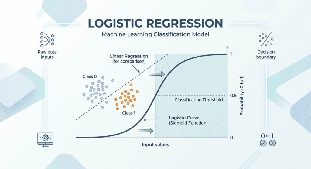
Linear regression struggles in a few specific situations. When the relationship between features and the target is clearly nonlinear, you’re better off with polynomial regression or a tree-based model. When you have a large number of correlated features, Ridge regression is the better starting point. When your target is categorical rather than continuous, linear regression is the wrong algorithm entirely — that’s what logistic regression handles.

And when your dataset is very small relative to the number of features you want to include, regularized versions are safer than plain OLS. The Gauss-Markov guarantee doesn’t save you when the training set is so small that the coefficient estimates are unstable regardless of the method.

FAQ

---

Linear regression is worth understanding deeply precisely because it’s so transparent. Every other algorithm you’ll learn is, at some level, trying to solve problems that linear regression can’t handle. Knowing exactly what those limits are, and what the math guarantees when you’re inside them, is what separates someone who runs model.fit() from someone who trusts the output.