Random Forest Algorithm Explained: Intuition & Python
Here’s the myth that gets repeated in almost every Random Forest tutorial: the algorithm works because many trees vote together and the majority vote is more accurate than any single tree.
That’s not wrong exactly, but it’s so incomplete it leads people to draw the wrong conclusions. If “many trees voting” were the full story, you could just train the same decision tree fifty times and average the results. It wouldn’t work. The trees would all look nearly identical because they’d be trained on the same data, making the same splits, and the vote would reflect one opinion repeated fifty times rather than fifty different perspectives.
The reason Random Forest actually works comes down to a specific mathematical constraint that Leo Breiman identified in his 2001 paper: the generalization error of a forest depends on two things simultaneously — how accurate the individual trees are, and how correlated those trees are with each other. The algorithm is specifically engineered to manage both. Understanding that dual constraint is the difference between knowing what Random Forest does and understanding why it works.
Table of Contents
From Decision Trees to an Ensemble
If you’ve worked through decision tree algorithms, you already know the fundamental problem: a single deep decision tree has high variance. Split the training data two different ways, train a tree on each half, and you often get dramatically different models. The tree is highly sensitive to which exact samples it sees.
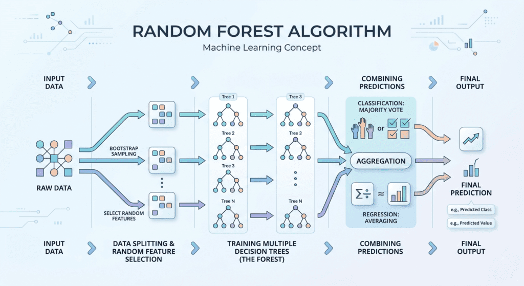
Bagging — short for bootstrap aggregating, introduced by Breiman in 1996 — was the first serious answer to this. The mechanism is straightforward: instead of training one model on your full dataset, you generate many bootstrap samples by sampling your training data with replacement, train a separate decision tree on each sample, and then aggregate their predictions by averaging (for regression) or majority vote (for classification).
Why does averaging help? If you have B independent estimates of the same quantity, each with variance σ², their average has variance σ²/B. As B grows, variance collapses toward zero. The weak law of large numbers guarantees it. The problem is that decision trees trained on bootstrap samples of the same dataset aren’t independent — they’re correlated. And once correlation enters the picture, the math changes in a critical way.
The variance of an average of B correlated estimates with pairwise correlation ρ is:
Var(average) = ρ·σ² + (1-ρ)·σ²/BThe second term vanishes as B increases. The first term doesn’t. If all trees are highly correlated — say ρ is close to 1 — averaging them does almost nothing for variance. You’re left with roughly σ² regardless of how many trees you build.
This is the problem bagging alone doesn’t fully solve. If your dataset has one very dominant predictive feature, every bootstrap sample will produce a tree that splits on that feature near the root. The trees look different superficially but are structurally similar. Their correlation stays high and the variance reduction from averaging is modest.
The Random Feature Selection Step That Changes Everything
Random Forest adds one crucial modification on top of bagging: at each split in each tree, instead of considering all available features, only a random subset of features — typically √p for classification and p/3 for regression, where p is the total number of features — is considered for the split.
This is the mtry parameter. It’s the part most tutorials mention once and move on from. It deserves more attention.
By restricting which features each tree can use at each node, you force trees to find different split paths through the data. A tree that can’t rely on the dominant feature at a given node has to find the next best thing. This produces structurally different trees — trees that are individually weaker but, critically, less correlated with each other. The ρ term in the variance equation drops, and averaging starts to work properly.
Breiman’s 2001 paper formalizes this precisely: the generalization error of a Random Forest is bounded by a function that increases with tree correlation and decreases with tree strength. The art of the algorithm is threading the needle between these two forces. Setting mtry low creates very uncorrelated trees (good for variance) but makes each tree individually weak (bad for strength). Setting mtry high makes trees stronger but more correlated. The default values (√p for classification) represent decades of empirical evidence about where that tradeoff typically lands.
A 2024 paper from researchers at MIT’s Operations Research Center took this further, showing that random feature subsets also reduce bias in certain high signal-to-noise settings — not just variance. The standard textbook explanation attributes Random Forest’s improvements entirely to variance reduction. The reality is that mtry is doing more than that, particularly when there are structured patterns that bagging alone would miss.
Out-of-Bag Error: Free Cross-Validation Built Into the Algorithm
When you create a bootstrap sample by sampling with replacement from N training examples, any given sample has a probability of (1 – 1/N)^N of never being selected. As N grows large, this converges to 1/e ≈ 0.368. In practice, roughly 36.8% of your training data is left out of each bootstrap sample.
These are the out-of-bag samples for that tree. They’ve never been seen by that tree during training. You can use them for validation.
For each training example, some fraction of trees in the forest were trained without it. You can make a prediction for that example using only those trees — its personal out-of-bag committee — and compare that prediction to the true label. The out-of-bag error is the aggregate of these predictions across all training examples.
What makes this significant isn’t the concept — it’s that it’s completely free. You’re not doing any additional training. You’re not holding out a validation set. You’re using data that was already left out as a byproduct of the bootstrap sampling process. Breiman proved this is an unbiased estimate of the generalization error as the number of trees grows.
In practice, this means you get a reliable accuracy estimate during training itself, which makes the hyperparameter tuning loop tighter: you can watch OOB error as you adjust n_estimators or max_depth without touching your held-out test set.
from sklearn.ensemble import RandomForestClassifier
from sklearn.datasets import make_classification
import numpy as np

X, y = make_classification(n_samples=1000, n_features=20, random_state=42)

rf = RandomForestClassifier(
    n_estimators=200,
    max_features='sqrt',     # mtry — random subset size per split
    oob_score=True,          # compute out-of-bag estimate during training
    n_jobs=-1,
    random_state=42
)
rf.fit(X, y)

print(f"OOB Accuracy: {rf.oob_score_:.4f}")
How to Implement Random Forest in scikit-learn
Most tutorials show you Random Forest code embedded inside a longer example. Here is the complete, self-contained implementation for both classification and regression so you have a clean reference.
RandomForestClassifier
Use this when your target variable is a category — spam vs not spam, churn vs retained, disease vs healthy.
from sklearn.ensemble import RandomForestClassifier
from sklearn.datasets import make_classification
from sklearn.model_selection import train_test_split
from sklearn.metrics import accuracy_score, classification_report

# Generate sample data
X, y = make_classification(
    n_samples=1000,
    n_features=20,
    n_informative=10,
    random_state=42
)

X_train, X_test, y_train, y_test = train_test_split(
    X, y, test_size=0.2, random_state=42
)

# Train the classifier
clf = RandomForestClassifier(
    n_estimators=300,       # number of trees
    max_features='sqrt',    # features considered per split (default for classification)
    max_depth=None,         # grow fully unpruned trees
    oob_score=True,         # use out-of-bag samples for a free accuracy estimate
    n_jobs=-1,              # use all CPU cores
    random_state=42
)
clf.fit(X_train, y_train)

# Evaluate
y_pred = clf.predict(X_test)
print(f"Test Accuracy:  {accuracy_score(y_test, y_pred):.4f}")
print(f"OOB Accuracy:   {clf.oob_score_:.4f}")
print(classification_report(y_test, y_pred))
The oob_score_ gives you a reliable accuracy estimate from training itself — no need to touch your test set during development. In most cases it tracks closely with cross-validation accuracy at a fraction of the compute cost.
RandomForestRegressor
Use this when your target variable is continuous — house prices, temperature, sales volume.
from sklearn.ensemble import RandomForestRegressor
from sklearn.datasets import make_regression
from sklearn.metrics import mean_squared_error, r2_score
import numpy as np

# Generate sample data
X, y = make_regression(
    n_samples=1000,
    n_features=20,
    n_informative=10,
    noise=0.1,
    random_state=42
)

X_train, X_test, y_train, y_test = train_test_split(
    X, y, test_size=0.2, random_state=42
)

# Train the regressor
reg = RandomForestRegressor(
    n_estimators=300,
    max_features=1/3,       # rule of thumb for regression: p/3 features per split
    max_depth=None,
    oob_score=True,
    n_jobs=-1,
    random_state=42
)
reg.fit(X_train, y_train)

# Evaluate
y_pred = reg.predict(X_test)
rmse = np.sqrt(mean_squared_error(y_test, y_pred))
print(f"RMSE:   {rmse:.4f}")
print(f"R²:     {r2_score(y_test, y_pred):.4f}")
print(f"OOB R²: {reg.oob_score_:.4f}")
One practical note: RandomForestRegressor does not predict outside the range of values it was trained on. If your training data spans house prices from $100k to $800k, the model will never predict $900k even for extreme inputs. For extrapolation tasks, gradient boosting or linear models are better suited.
Random Forest Feature Importance: What It Measures and Where It Misleads
Random Forest computes feature importance as a natural byproduct of training — you don’t need a separate analysis pass. There are two methods, and they work differently.
Mean Decrease Impurity (MDI) totals up the weighted reduction in Gini impurity (or variance, for regression) produced by each feature across all splits in all trees, then normalizes. Features that produce larger purity improvements when split on get higher scores. This is fast to compute and available by default via feature_importances_ in scikit-learn.
Permutation importance works differently, and Breiman built it into the original Random Forest algorithm using OOB samples. For each feature, you randomly shuffle its values in the OOB set (breaking any real relationship between that feature and the target), then measure how much the OOB accuracy drops. A large drop means the feature was doing real work. A small drop means the model didn’t rely on it much.
The research here is worth knowing. A 2007 paper by Strobl and colleagues published in BMC Bioinformatics showed that MDI is systematically biased in favor of features with many unique values (high cardinality). A continuous feature with many possible split points gets artificially inflated importance relative to a binary feature, even when their predictive power is similar. Scikit-learn’s documentation explicitly acknowledges this.
Permutation importance doesn’t have this cardinality bias, but it has a different issue: when features are correlated with each other, permuting one of them partially breaks the model’s access to its correlated partners, causing the importance of all correlated features to be underestimated. There’s no clean solution. The right answer is to use both methods and look for agreement, and to interpret any importance score as relative and directional rather than as a precise causal measure.
import pandas as pd
from sklearn.inspection import permutation_importance

# Permutation importance (on test set, not OOB)
result = permutation_importance(rf, X, y, n_repeats=10, random_state=42, n_jobs=-1)

importance_df = pd.DataFrame({
    'feature': [f'feature_{i}' for i in range(X.shape[1])],
    'mdi_importance': rf.feature_importances_,
    'permutation_importance': result.importances_mean
}).sort_values('permutation_importance', ascending=False)

print(importance_df.head(10))
Why It Consistently Wins on Tabular Data
A 2015 paper in the Annals of Statistics by Scornet, Biau and Vert proved the consistency of Breiman’s original Random Forest algorithm for additive regression models — meaning as data grows, the forest’s predictions converge to the true underlying function. The proof also revealed something practically useful: Random Forest adapts naturally to sparsity in the feature space. When most features are irrelevant, the algorithm still finds the informative ones, because random feature selection repeatedly gives those features chances to demonstrate their predictive value across many trees.
This theoretical result lines up with practical observation across decades of Kaggle competitions, industry applications, and academic benchmarks. Random Forest regularly outperforms more complex algorithms on tabular data with limited preprocessing. It’s been the winning model in applications from air quality forecasting to clinical outcome prediction to ecological species distribution modelling.
The practical reasons compound the theoretical ones. Random Forest requires minimal preprocessing — no feature scaling, reasonably robust to outliers, handles mixed feature types without manual encoding tricks. Each tree is trained independently, making the algorithm embarrassingly parallelizable. You can double the number of trees and the training time stays the same if you have the cores for it.
It’s also notably resistant to overfitting as you add more trees, unlike many algorithms where additional capacity without regularization leads to worse generalization. Adding trees past a certain point produces diminishing returns, but it doesn’t hurt. This stability makes it forgiving during the tuning phase.
Random Forest Hyperparameters: What Actually Matters
Most of the twenty-plus parameters in scikit-learn’s RandomForestClassifier can be left at defaults and you’ll get a reasonable model. Three parameters genuinely matter for most applications.
n_estimators controls how many trees to build. More trees is almost always better up to a point — OOB error typically stabilizes between 100 and 500 trees depending on dataset complexity. Beyond that, you’re spending compute without measurable accuracy gains. Start at 300 and check your OOB error curve.
max_features (the mtry analog) controls how many features are randomly considered at each split. The default of sqrt for classification is a strong prior based on extensive empirical research. If you’re getting poor performance, try values from max_features=2 up to max_features=p (which degenerates to pure bagging with no feature randomization).
max_depth limits how deep each tree can grow. Breiman’s original algorithm grows fully unpruned trees. The consistency proof assumes this. In practice, limiting depth with small datasets can reduce overfitting, but for most medium-to-large tabular datasets the defaults are sensible.
from sklearn.model_selection import cross_val_score

rf_tuned = RandomForestClassifier(
    n_estimators=300,
    max_features='sqrt',    # default, based on Breiman's recommendation
    max_depth=None,         # fully grown trees per original algorithm
    min_samples_leaf=1,
    oob_score=True,
    n_jobs=-1,
    random_state=42
)

cv_scores = cross_val_score(rf_tuned, X, y, cv=5, scoring='accuracy')
print(f"CV Accuracy: {cv_scores.mean():.4f} ± {cv_scores.std():.4f}")
Real-World Use Cases for Random Forest
Random Forest became a go-to algorithm across industries not because it is the most sophisticated model available, but because it consistently produces reliable predictions on structured data with minimal preprocessing and a short path from raw data to working model. Here are the domains where it appears most frequently in production.
Fraud Detection
Banks and payment processors use Random Forest to flag suspicious transactions in real time. The algorithm handles the heavily imbalanced class distribution typical in fraud data (fraudulent transactions are often less than 1% of the total), and its ensemble nature makes it resistant to outlier transactions that might fool a single model. Features like transaction velocity, geographic anomalies, and device fingerprints combine in ways that are difficult to express as explicit rules but straightforward for a forest to learn from examples.
Credit Scoring and Loan Risk
Credit underwriting involves dozens of correlated features — income, employment history, existing debt, payment records — and Random Forest’s built-in feature importance provides a natural audit trail for which factors drove a given risk score. Regulatory requirements in many markets require explainability, and while a full forest is not interpretable at the prediction level, aggregate feature importances satisfy many compliance reviews at the model level.
Medical Diagnosis and Clinical Outcome Prediction
Clinical datasets are often medium-sized (thousands to tens of thousands of patients), high-dimensional (hundreds of biomarkers or imaging features), and noisy. Random Forest performs well in this regime. Published applications include predicting sepsis risk from ICU time-series data, classifying tumor types from gene expression profiles, and estimating readmission probability from electronic health records. The OOB error estimate is particularly useful here since holding out a separate validation set from a small clinical dataset reduces training data meaningfully.
Demand Forecasting and Inventory Planning
Retailers and supply chain teams use Random Forest regressors to forecast product demand across time. Inputs typically include historical sales, promotions, seasonality indicators, local events, and weather data. The algorithm handles the mixed feature types and nonlinear relationships between them without requiring the extensive feature engineering that linear models need to capture the same patterns.
Feature Selection and Preprocessing Pipelines
Before training a more complex model, teams often run a Random Forest first specifically to use its feature importances for dimensionality reduction. Features scoring below a threshold are dropped from the final modeling dataset. This is sometimes called a “permutation importance filter.” It’s computationally cheap relative to wrapper methods like recursive feature elimination, and it has a solid theoretical basis in how Random Forest identifies informative features across many bootstrap samples.
When to Move Beyond Random Forest
Random Forest isn’t always the right call, and knowing when to step past it is as important as knowing when to reach for it.
If your dataset is very large (millions of rows), gradient boosting methods — XGBoost, LightGBM, CatBoost — often outperform Random Forest both in accuracy and training time. They build trees sequentially, each correcting the residual errors of the previous, which can get more from fewer trees. The tradeoff is more hyperparameters and more sensitivity to overfitting. A detailed comparison of when to switch is in the gradient boosting guide.
For high-dimensional datasets where the number of features substantially exceeds the number of samples — genomics, text features, some image pipelines — Random Forest’s random feature subsets help but may not be enough. Specialized methods or dimensionality reduction preprocessing often outperform it in those settings.
And if you need calibrated probability estimates, be aware that Random Forest’s out-of-the-box probabilities (proportion of trees voting for each class) are known to be poorly calibrated, particularly near 0 and 1. Platt scaling or isotonic regression post-processing is worth considering before using the probabilities for decision-making.
The scikit-learn RandomForestClassifier documentation covers parameter options, solver details, and worked examples thoroughly.
Random Forest vs Decision Tree: When to Use Each
A single decision tree and a Random Forest are solving the same problem — splitting a feature space to predict an outcome — but they make opposite tradeoffs. Knowing which tradeoff fits your situation is more useful than memorizing that “Random Forest is better.”
| Property | Decision Tree | Random Forest |
|---|---|---|
| Variance | High — small data changes produce very different trees | Low — averaging across 100s of trees smooths instability |
| Bias | Low (when fully grown) | Slightly higher — random feature subsets mean individual trees are weaker |
| Overfitting risk | High on complex datasets | Low — bagging and feature randomization both push against it |
| Interpretability | High — you can read a single path from root to leaf | Low — no single tree represents the forest’s decision logic |
| Training time | Fast | Slower — scales linearly with n_estimators, but parallelizable |
| Prediction speed | Fast | Slower — each prediction queries all trees |
| Feature importance | Available, but unstable across reruns | Available and stable — averaged across all trees |
| Handles missing values | Needs imputation | Needs imputation (scikit-learn implementation) |
| Minimum viable dataset size | Works on small datasets | Benefits from at least a few hundred samples to bootstrap meaningfully |
The core rule: if you need to explain a specific prediction to a non-technical stakeholder, a pruned decision tree is often the right call. If you need maximum predictive accuracy and interpretability is secondary, Random Forest is almost always the better starting point.
One place the decision tree genuinely wins beyond interpretability: when you have a very small dataset (under 200–300 samples), bootstrap sampling may actually hurt you. Each bootstrap sample leaves out roughly 37% of your data, which means individual trees in the forest see even less data than you have. A carefully pruned single tree trained on your full dataset can outperform a forest in that regime.
For a deeper walkthrough of how decision trees build their splits, see the decision tree algorithm guide.
FAQ
What is Random Forest and how does it work?
Random Forest is an ensemble learning algorithm that trains many decision trees on different bootstrap samples of the training data and aggregates their predictions. The key addition beyond simple bagging is that at each split within each tree, only a random subset of features is considered. This random feature selection reduces the correlation between trees, which is the mechanism that makes averaging predictions genuinely effective rather than redundant.
What is the difference between Random Forest and a decision tree?
A single decision tree is high-variance: small changes in training data produce very different trees. It’s also interpretable and fast to train. Random Forest sacrifices interpretability to buy variance reduction: by training many trees on different bootstrap samples with random feature subsets and averaging their predictions, it produces a model that’s substantially more stable and typically more accurate on unseen data. The cost is that you lose the ability to read a single logical tree path and explain a prediction directly.
How does feature importance work in Random Forest?
Random Forest provides two built-in approaches. Mean Decrease Impurity (MDI) measures how much each feature reduces impurity across all splits in all trees — fast but biased toward high-cardinality features. Permutation importance shuffles each feature’s values in the out-of-bag set and measures the resulting accuracy drop — more reliable for ranking but sensitive to correlated features. Research by Strobl et al. (2007) documented the MDI cardinality bias explicitly; for feature selection decisions, permutation importance is the more trustworthy of the two.
How many trees should a Random Forest have?
Enough that the out-of-bag error has stabilized. In practice this is usually somewhere between 100 and 500 trees for typical tabular datasets. A useful diagnostic is to plot OOB accuracy against n_estimators during training and look for where the curve flattens. Unlike most algorithm parameters, adding more trees past the stability point doesn’t cause overfitting — it just wastes compute. Start at 300 and adjust based on your OOB error curve.