Your Gradient Boosting Model Is Overfitting — Here’s Exactly Why (and How to Fix It)

Training accuracy: 98%. Test accuracy: 71%. Sound familiar?

If you built a gradient boosting model that performs brilliantly on training data and collapses on anything new, you are hitting the most common trap in the algorithm. The frustrating part is that gradient boosting is supposed to be one of the most powerful tools for tabular data — and it is. The same property that makes it powerful is exactly what makes it overfit.

This guide covers what causes gradient boosting to overfit, three proven fixes you can apply in scikit-learn, and the order to try them in. Every fix comes with working Python code. No theory for theory’s sake.

If you are new to the algorithm itself, start with how gradient boosting works for beginners first, then come back here.

Why Gradient Boosting Overfits in the First Place

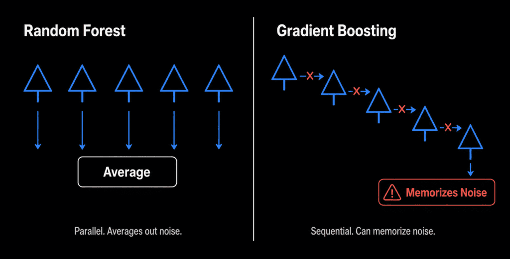
To understand why gradient boosting overfits, you need to see how it differs from something like random forest.

Random forest builds hundreds of decision trees independently and in parallel. Each tree sees a slightly different slice of the data. The final prediction averages their outputs. That averaging naturally smooths out noise — it is variance reduction by design.

Gradient boosting takes the opposite approach. It builds trees sequentially. Tree one makes predictions. Tree two looks at where tree one was wrong and tries to correct those mistakes. Tree three corrects what tree two missed. Each tree is completely aware of every error the previous trees made.

This sequential correction is what makes gradient boosting so accurate on tabular data. It is also what makes it overfit. When you have too many trees, or when each tree is allowed to grow too deep, the model stops learning genuine patterns. Instead, it starts memorizing specific quirks in your training data — including random noise that will never appear in new data.

Three parameters control this behavior: learning rate, tree depth, and the number of trees (n_estimators). Getting these right is the entire job of fixing overfitting in gradient boosting.

Fix 1: Reduce the Learning Rate

The learning rate is the single most important parameter for controlling overfitting in gradient boosting.

Every time a new tree is added to the ensemble, its predictions are scaled by the learning rate before being added to the running total. A learning rate of 1.0 means each tree contributes its full weight. A rate of 0.1 means each tree contributes only 10% of its prediction.

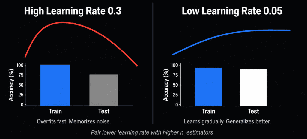
Lower learning rate means each individual tree has less influence. The model needs more trees to reach the same accuracy level, which forces it to learn more gradually and generalize better. Research by Jerome Friedman — the statistician who formalized the gradient boosting algorithm — showed that learning rates below 0.1 paired with a sufficient number of trees consistently outperform high learning rates, even when overall training time is controlled for (Friedman, 2001).

Most practitioners start at 0.1. If your model is overfitting, try 0.05 or 0.01. The tradeoff is training time: a lower learning rate requires more trees, so increase n_estimators alongside it. (Fix 3 below handles this automatically with early stopping.)

from sklearn.ensemble import GradientBoostingClassifier
from sklearn.model_selection import train_test_split
from sklearn.metrics import accuracy_score

X_train, X_test, y_train, y_test = train_test_split(
    X, y, test_size=0.2, random_state=42
)

# Before: High learning rate — likely overfitting
model_overfit = GradientBoostingClassifier(
    learning_rate=0.3,
    n_estimators=100,
    random_state=42
)
model_overfit.fit(X_train, y_train)

# After: Lower learning rate with more trees
model_fixed = GradientBoostingClassifier(
    learning_rate=0.05,
    n_estimators=300,
    random_state=42
)
model_fixed.fit(X_train, y_train)

print("Overfit model test accuracy:", accuracy_score(y_test, model_overfit.predict(X_test)))
print("Fixed model test accuracy:", accuracy_score(y_test, model_fixed.predict(X_test)))

A good working range for learning rate is 0.01 to 0.2. Values above 0.3 are almost always too high for production use — they are fine for quick prototyping but not for a model you actually want to generalize.

Fix 2: Reduce Tree Depth

The learning rate controls how much each tree contributes. Tree depth controls how complex each individual tree is allowed to get.

Scikit-learn’s default max_depth is 3, which is already a shallow tree. A depth-3 tree can capture up to three-way feature interactions — for example, “age AND income AND education level.” That is enough for most tabular problems. Increasing depth lets the model capture more complex patterns, which sounds useful. The downside is that deeper trees also fit noise. A depth-8 tree can memorize very specific combinations in your training data that will never appear in new data.

For most problems, a max_depth between 3 and 5 works well. If your model is still overfitting after reducing the learning rate, drop max_depth to 3 and measure whether test performance improves.

python

from sklearn.ensemble import GradientBoostingClassifier

model = GradientBoostingClassifier(
    learning_rate=0.05,
    n_estimators=300,
    max_depth=3,          # Shallow trees — reduces overfitting
    min_samples_leaf=10,  # Each leaf needs at least 10 samples
    random_state=42
)
model.fit(X_train, y_train)

min_samples_leaf is worth adding at the same time. It sets the minimum number of training samples required at a leaf node. Increasing it prevents the model from creating tiny, highly specific leaf nodes that only exist to memorize one or two training examples. A value of 10 to 20 works well for most datasets.

To understand why shallow trees help here, it is the same reason they work in decision trees for beginners — depth controls the bias-variance tradeoff, and for gradient boosting, you want to keep individual trees biased toward simplicity.

Fix 3: Use Early Stopping

Early stopping is the most practical fix of the three, because it removes the guesswork from choosing n_estimators entirely.

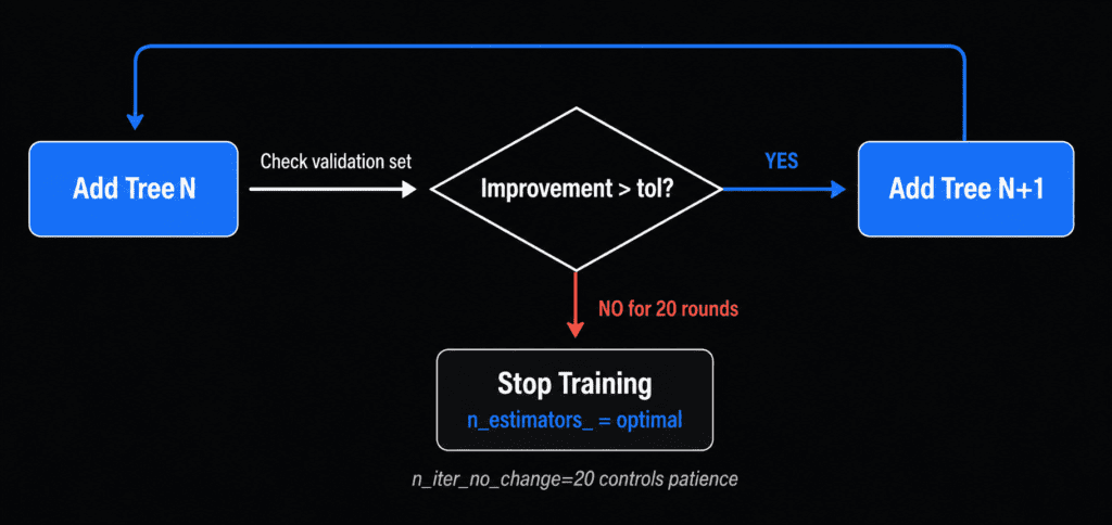
Here is how it works. You set aside a small validation set during training. After each new tree is added, gradient boosting checks performance on this validation set. When validation performance stops improving for a set number of consecutive rounds — controlled by n_iter_no_change — training halts automatically.

You no longer need to guess how many trees to use. Set a large upper bound for n_estimators (say, 1000), enable early stopping, and let the algorithm find the right stopping point on its own.

from sklearn.ensemble import GradientBoostingClassifier
from sklearn.metrics import accuracy_score

model = GradientBoostingClassifier(
    learning_rate=0.05,
    n_estimators=1000,          # High upper bound — early stopping handles the rest
    max_depth=3,
    validation_fraction=0.1,    # Hold out 10% of training data for validation
    n_iter_no_change=20,        # Stop if no improvement for 20 consecutive rounds
    tol=1e-4,
    random_state=42
)
model.fit(X_train, y_train)

print(f"Training stopped at: {model.n_estimators_} trees")
print("Test accuracy:", accuracy_score(y_test, model.predict(X_test)))

The n_iter_no_change value of 20 is a solid default. Lower values stop training earlier and are more conservative. Higher values let training continue longer, which can help find late performance gains on larger datasets.

This approach aligns with how practitioners use gradient boosting in real production settings — Google’s machine learning course on gradient boosted decision trees recommends combining shrinkage (learning rate) with early stopping as the primary regularization strategy (Google for Developers).

Bonus Fix: Add Subsampling

This fix is less commonly taught but has strong research backing.

Friedman’s 2002 paper on stochastic gradient boosting found that training each tree on a random subset of the training data — rather than the full dataset — often produces better generalization than using all the data (Friedman, 2002). A subsample value of 0.5 frequently outperforms 1.0, even though each tree sees less data.

The reason is the same mechanism that makes bagging work: introducing randomness decorrelates successive trees and reduces variance. This variant is called stochastic gradient boosting.

model = GradientBoostingClassifier(
    learning_rate=0.05,
    n_estimators=1000,
    max_depth=3,
    subsample=0.8,              # Each tree trains on 80% of the data
    validation_fraction=0.1,
    n_iter_no_change=20,
    random_state=42
)
model.fit(X_train, y_train)

A subsample value between 0.5 and 0.9 is typical. Going below 0.5 introduces too much variance and can hurt performance. This fix pairs especially well with a lower learning rate — together they are the two strongest levers for getting gradient boosting to generalize properly.

The Order to Apply These Fixes

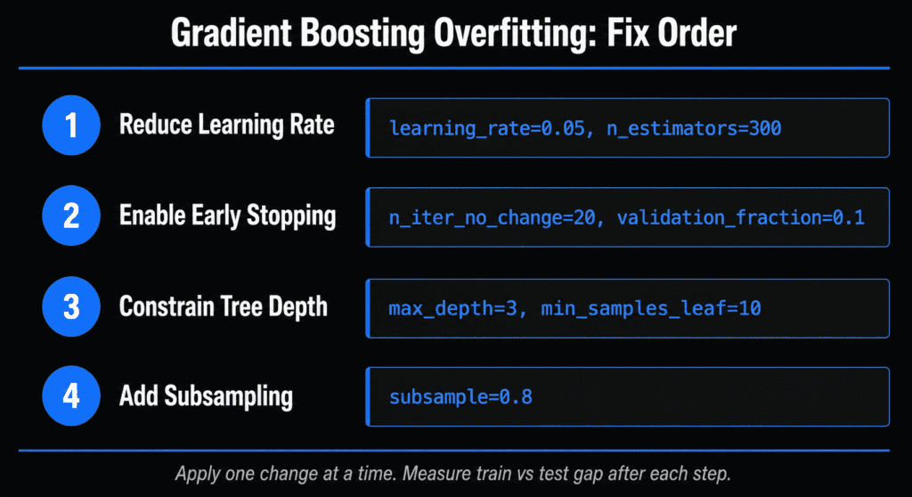
Do not adjust all parameters at once. You will lose track of what is actually helping. A practical sequence:

Start by reducing the learning rate to 0.05 and increasing n_estimators to 300. Measure the gap between training and test accuracy. Next, enable early stopping with n_iter_no_change=20 to find the true optimal tree count automatically. If overfitting persists, reduce max_depth to 3 and add min_samples_leaf=10. Finally, add subsample=0.8 as the last step.

Stop when the gap between training and test accuracy is small enough for your use case. You do not need perfect symmetry — some gap is normal and expected.

To know whether your fixes actually worked, you need the right evaluation metrics. How to evaluate a machine learning model walks through accuracy, precision, recall, and when each one matters.

Frequently Asked Questions

Why does gradient boosting overfit so easily?

Gradient boosting builds trees sequentially, with each tree correcting the errors of the previous one. Without constraints, it keeps fitting residuals until it memorizes training data noise — especially when the learning rate is high or the number of trees is large. It has no built-in randomness like random forest does.

What is the best learning rate for gradient boosting?

There is no single best value. Start between 0.05 and 0.1 for most problems. Pair a lower learning rate with a higher n_estimators and use early stopping to find the optimal tree count automatically rather than guessing.

How does early stopping prevent overfitting in gradient boosting?

It monitors a held-out validation set after each boosting round and halts training when performance stops improving. This prevents the model from adding trees that only improve training accuracy while hurting test accuracy. It also removes the need to manually tune n_estimators.

Should I fix learning rate or tree depth first?

Fix learning rate first — it has the biggest impact on overfitting. Once stabilized, reduce max_depth (try 3 to 5) if the model is still memorizing the training data.

Is gradient boosting more prone to overfitting than random forest?

Yes, generally. Random forests build trees independently and average their results, which reduces variance by design. Gradient boosting’s sequential correction makes it more accurate on complex problems but more sensitive to hyperparameter choices — which is why tuning matters more than it does for random forest.

Summary

Gradient boosting overfits because its sequential learning has no built-in variance reduction. The model keeps correcting errors until it memorizes the training data. Three parameters control this: learning rate, tree depth, and number of trees.

Start with learning rate and early stopping — they cover most cases. Add tree depth constraints and subsampling if overfitting persists. Always measure the gap between training and test accuracy after each change to know whether the fix actually worked.

Ready to go further? Ensemble learning explained for beginners covers the foundation of how boosting, bagging, and stacking relate to each other. For a side-by-side comparison of when to pick gradient boosting versus random forest, see gradient boosting vs random forest: which should you use?.

Sources: Friedman, J.H. (2001). Greedy function approximation: A gradient boosting machine. Annals of Statistics, 29(5). | Friedman, J.H. (2002). Stochastic gradient boosting. Computational Statistics & Data Analysis. | Google for Developers. Introduction to Gradient Boosted Decision Trees. | scikit-learn. GradientBoostingClassifier documentation.