Support Vector Machines Explained: The Algorithm Nobody Explains Well

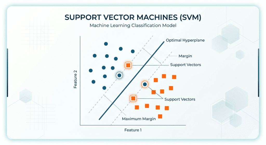
The first time someone explained Support Vector Machines to me, they drew a line between two clusters of dots on a whiteboard and said “the SVM finds the best line.” I nodded. I had no idea what made one line better than another, why any of this was useful when the data wasn’t separable by a line, or what a “kernel” was doing in a classification algorithm.

Most SVM explanations stop at that whiteboard level. They define the hyperplane, mention something called a kernel, show you a code snippet, and move on. What they skip is the actual reasoning that makes SVMs work — and why the geometric insight behind them is genuinely elegant in a way that most algorithms aren’t.

This post works through SVMs from the research up. I’m drawing directly from Cortes and Vapnik’s 1995 paper in Machine Learning that introduced the modern SVM, the 1992 Boser-Guyon-Vapnik paper that brought the kernel trick, and a 2020 empirical study by Wainer and Fonseca that tested C and gamma tuning across 115 real datasets. The goal is to give you the understanding that the whiteboard explanation skipped.

What a Support Vector Machine Is Actually Doing

A Support Vector Machine is a supervised classification algorithm that finds the decision boundary between classes with the largest possible margin. That sentence has a specific mathematical meaning that’s worth unpacking.

Definition: A Support Vector Machine constructs a hyperplane (or set of hyperplanes) in feature space that separates classes by the maximum possible margin. The margin is defined as the distance from the decision boundary to the nearest training point on either side. Maximizing this margin minimizes the generalization error, meaning the model is less likely to misclassify new, unseen points.

The term hyperplane sounds more intimidating than it is. In two dimensions, a hyperplane is a line. In three dimensions, it’s a flat plane. In higher dimensions, it’s the n-1 dimensional surface that divides the space. The SVM finds the particular hyperplane that sits as far as possible from the training points nearest to it on each side.

Those nearest points are what give the algorithm its name: they are the support vectors. They are the only training examples that actually determine where the decision boundary sits. Remove a training point that isn’t a support vector, retrain the model, and you get the exact same boundary. This sparsity property is one of SVMs’ genuine advantages: after training, most of your data is irrelevant to the model’s predictions.

Why does maximizing the margin help? Cortes and Vapnik’s 1995 paper demonstrated this through VC theory — the mathematical framework for measuring a model’s capacity to overfit. The core result is that a wider margin corresponds to lower model capacity, which means better generalization to unseen data. A decision boundary crammed close to training points has memorized where those specific points sit. A boundary with a wide margin on both sides has room for the class boundary to shift slightly and still classify correctly.

The Soft Margin: How SVMs Handle Real Data

The original SVM formulation worked only when the data was linearly separable, meaning a hyperplane could perfectly divide the classes with no mistakes. Real data almost never cooperates.

The 1995 Cortes-Vapnik paper introduced the soft margin precisely to handle this. The soft margin allows some training points to be on the wrong side of the decision boundary during training, but penalizes those violations. This is where the regularization C parameter enters.

C controls how much you care about misclassifying training points versus how wide you want the margin to be. A large C says: “penalize mistakes heavily, shrink the margin if you have to, just get the training points right.” A small C says: “accept some training errors, keep the margin wide, don’t overfit.”

The research from Wainer and Fonseca (2020) makes this concrete. Studying 115 real binary classification datasets, they confirmed that C functions as an inverse regularization term: a lower C allows more support vectors and results in larger margins, while a higher C pushes the model toward fewer support vectors but tighter fit to training data. Their practical finding aligns with what the scikit-learn team documents: when multiple pairs of C and gamma give equivalent cross-validation accuracy, prefer the smaller C. Lower C reduces fitting time and avoids unnecessary complexity.

The Kernel Trick: Why SVMs Work on Non-Linear Problems

Here’s where most explanations wave their hands and say “the kernel trick maps data into a higher-dimensional space.” That’s true, but it hides the part that’s actually interesting.

When data isn’t linearly separable in its original feature space, you can sometimes find a transformation φ(x) that maps it into a higher-dimensional space where it becomes separable. The SVM then finds a hyperplane in that high-dimensional space.

The problem is that explicitly computing φ(x) for every point can be astronomically expensive. If you’re mapping into thousands of dimensions, this is often impossible in practice.

The insight from Boser, Guyon, and Vapnik (1992) is that you never actually need to compute φ(x) explicitly. The SVM optimization problem only ever needs the dot products between pairs of transformed points: φ(xᵢ)ᵀ φ(xⱼ). And for many useful transformations, you can compute this dot product in the original feature space using a kernel function K(xᵢ, xⱼ), without computing the individual φ(x) values at all.

K(xᵢ, xⱼ) = φ(xᵢ)ᵀ φ(xⱼ)

You never go to the high-dimensional space. You compute similarity between points in the original space using the kernel, and the math works out as if you had. This is what “kernel trick” actually means: implicit computation in a space you never have to visit.

The RBF Kernel and How to Think About Gamma

The most commonly used kernel in practice is the RBF kernel (Radial Basis Function), defined as:

K(xᵢ, xⱼ) = exp(−γ ||xᵢ − xⱼ||²)

The kernel value between two points drops off as they get farther apart, controlled by γ. Think of γ as defining how “local” the model’s memory is. A high γ means the kernel value drops off steeply with distance, so each support vector only influences predictions near it — the decision boundary becomes very wiggly and local. A low γ means the influence of each support vector spreads far, producing smoother decision boundaries.

In practice, γ and C interact. According to the scikit-learn documentation on RBF SVM parameters, once C is large enough that there are no more training violations, the RBF kernel alone acts as a structural regularizer — increasing C further stops helping. Their documentation puts it this way: the gamma parameter can be thought of as the inverse of the radius of influence of samples selected as support vectors.

The Wainer and Fonseca (2020) paper adds a useful practical finding: the joint optimization of C and γ is a non-convex problem. There is no single guaranteed path to the global best values. Their empirical comparison of 18 different search algorithms across those 115 datasets found that grid search, despite being the most basic approach, performs comparably to sophisticated optimization methods when given the same number of evaluations. Spending significantly more compute on fancier search procedures doesn’t reliably produce better test accuracy. The LibSVM package, which remains the most widely used SVM solver, uses a grid in the range 2⁻⁵ ≤ C ≤ 2¹⁵ and 2⁻¹⁵ ≤ γ ≤ 2³ as a practical default search space.

The implication: don’t overthink hyperparameter search for SVMs. A reasonable grid with 5-fold cross-validation gets you most of the way there.

from sklearn.svm import SVC
from sklearn.model_selection import GridSearchCV
from sklearn.preprocessing import StandardScaler
from sklearn.pipeline import Pipeline

pipe = Pipeline([
    ('scaler', StandardScaler()),           # critical — SVM is not scale-invariant
    ('svm', SVC(kernel='rbf'))
])

param_grid = {
    'svm__C':     [0.1, 1, 10, 100],
    'svm__gamma': [1e-3, 1e-2, 0.1, 1]
}

search = GridSearchCV(pipe, param_grid, cv=5, scoring='accuracy', n_jobs=-1)
search.fit(X_train, y_train)

print(f"Best C: {search.best_params_['svm__C']}")
print(f"Best gamma: {search.best_params_['svm__gamma']}")
print(f"Test accuracy: {search.score(X_test, y_test):.3f}")

Note the scaler. SVMs are not scale-invariant because the margin calculation depends on distances in feature space. If one feature runs from 0 to 1 and another from 0 to 10,000, the second feature dominates the distance calculation and the model sees a distorted picture of the data. Always scale before fitting an SVM.

Where SVMs Genuinely Outperform Other Algorithms

SVMs have a specific performance profile worth knowing, because they’re not the right tool for every problem.

They tend to perform exceptionally well on high-dimensional data with relatively few samples. Text classification is the canonical example: a document represented as a bag of words might have tens of thousands of features but only a few thousand documents. In this regime, logistic regression often struggles with multicollinearity and tree-based methods struggle with the sparsity. SVMs, because they only rely on a subset of training points (the support vectors) and compute similarity through kernels, handle this regime naturally.

The Cortes and Vapnik 1995 paper included a benchmark on Optical Character Recognition where the support vector network outperformed several classical approaches of the time. The 2020 Wainer and Fonseca study, across 115 more modern binary classification datasets, confirmed that SVM with an RBF kernel remains among the top two or three classifiers across diverse real-world data.

They are a harder sell when you have very large training datasets. The computational cost of SVM training scales poorly with sample size — roughly O(n²) to O(n³) depending on the solver. On 100,000 training examples, the training time becomes painful. On datasets that large, gradient-boosted trees or even logistic regression with regularization typically give comparable accuracy at a fraction of the training cost.

The other limitation is interpretability. SVMs don’t produce easily readable feature importances. You can identify which training examples are support vectors, but translating that back into “feature X matters because…” is not straightforward. For problems where model explainability is a requirement, logistic regression gives you probability outputs and interpretable coefficients that SVMs simply don’t.

The Practical Decision

SVMs reward you for understanding their geometry. The C parameter isn’t a magic dial — it’s the lever controlling where you sit on the bias-variance tradeoff within the soft margin formulation. The kernel trick isn’t a black box — it’s implicit computation in a space you never visit directly. And the support vectors are a specific, meaningful set of training points: if you removed everything else from your training data, you’d train the same model.

Understanding this makes tuning non-random. A model that’s memorizing the training data has a high γ and high C — both pulling toward complex, tightly-fit boundaries. A model that’s underfit has too low a γ or C — spreading influence too broadly or accepting too much slack. Grid search finds the crossing point, but knowing the geometry tells you which direction to push when results aren’t satisfying.

FAQ